22  Exponential discounting

Exponential discounting occurs when an agent discounts future costs and benefits at a consistent rate through time.

Under exponential discounting, each additional period of delay results in a discount of a future cost or benefit by a factor of \delta. The discount factor \delta is a number between 0 and 1. The higher the discount factor, the less the agent discounts future costs and benefits.

You will often see discussion of the ”discount rate”, r. In discrete time, the relationship between \delta and r is as follows:

\delta=\frac{1}{1+r}

A larger discount factor implies less discounting. A larger discount rate implies more discounting.

Under the standard model of exponential discounting, an agent with a choice between alternative streams of payoffs will seek to maximize the discounted utility of the future path of consumption.

The following equation is an example of exponential discounting, with a stream of costs or benefits x_0 through to x_T incurred at periods 0 through to T. U_0 is utility of the stream of payoffs at time t=0. x_t is the payoff in period t.

\begin{align*} U_0&=u(x_0)+\delta u(x_1)+\delta^2u(x_2)+\delta^3u(x_3)+...+\delta^Tu(x_T) \\[6pt] &=\sum_{t=0}^{t=T}\delta^tu(x_t) \\[12pt] 0&\leq \delta\leq1 \end{align*}

Each period of delay results in a discount of the future cost or benefit by a factor of \delta. One period of delay results in a discount of \delta. Two periods of delay results in a discount of \delta^2. Three periods of delay results in a discount of \delta^3 and so on.

The degree of discounting in this equation evolves each period as 1, \delta, \delta^2, \delta^3, \delta^4 and so on. This results in a smooth decline in present value of a future payoff over time.

22.1 Visualising exponential discounting

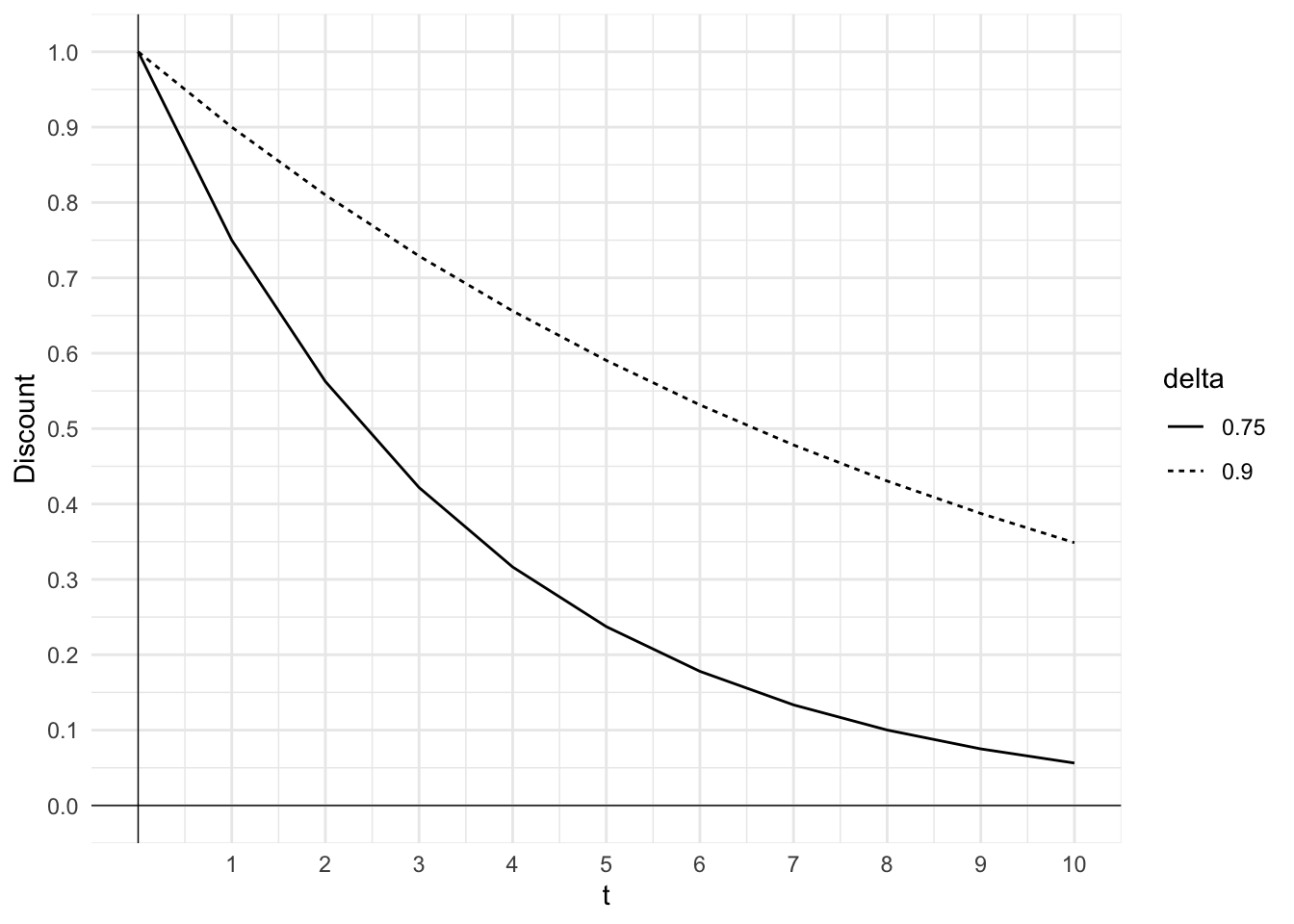
Figure 22.1 illustrates the effect of exponential discounting. The figure plots the size of the discount as a function of t for an exponential discounter with \delta=0.9 and \delta=0.75.

#Plot of exponential discounting with two curves, one with delta=0.9 and one with delta=0.75

##Load the ggplot2 package
library(ggplot2)
library(tidyr)

#Define the discount factor
delta <- c(0.75, 0.9)

#Define the number of periods
t <- 0:10

#Define the discount function
discount <- function(delta, t) {
  delta^t
}

#data frame with three rows: t, discount(0.75, t) and discount(0.9, t)
discounted <- data.frame(t, discount(delta[1], t), discount(delta[2], t))

colnames(discounted) <- c("t","0.75","0.9")

discounted <- pivot_longer(discounted, cols = -t, names_to = "delta", values_to = "discount")

#Plot the discount function with curves for each of the two values of delta using ggplot2
ggplot(discounted, aes(x=t, y=discount, group=delta, linetype=delta)) +
    geom_line() +
    labs(x="t", y="Discount") +
    theme_minimal() +
    scale_x_continuous(breaks=1:10) +
    scale_y_continuous(breaks=seq(0, 1, 0.1)) +
    geom_vline(xintercept = 0, linewidth=0.25)+ 
    geom_hline(yintercept = 0, linewidth=0.25)

Figure 22.1: Exponential discount curves

22.2 Exponential discounted utility model assumptions

The standard model of exponential discounting is underpinned by several assumptions.

22.2.1 Time-consistency

The first is time consistency.

Once the agent starts moving along the consumption path, they are time-consistent with their initial plan. For example, consider an agent facing the following two choices:

Would you like $100 today or $110 next week?

Would you like $100 next week or $110 in two weeks?

An exponential discounter will choose $100 in both choices or $110 in both choices. The reason is that after one week the second choice effectively becomes the same as the first choice. Time consistency implies that they will continue to want to make the same choice regardless of when they are making it.

22.2.2 Consumption independence

A second assumption is consumption independence.

Consumption independence means that utility in period t+k is independent of consumption in any other period. An outcome’s utility is unaffected by outcomes in prior or future periods.

Imagine a world where an exponential discounter intends to consume a behavioural economics subject.

Suppose that exponential discounter wants to consume lecture 1 at t+3 and lecture 2 at t+4. Under consumption independence, if the agent does not attend lecture 1, they still expect to benefit from lecture 2 at t+4 consistent with the plan they decided at t.

This assumption allows us to write x=x_1+x_2+x_3+...+x_n. That is, good x can be split, allocated and moved across periods without changing the value of that good beyond the effect of the discount.

22.2.3 Stationary preferences

A third assumption is stationary preferences.

That is, U_t=U_{t=K}.

The utility function is stationary across periods. The functional form of U_t is the same as the functional form of U_{t+k}.

That means that if someone likes ice cream today, they will get the same utility from ice cream at a future time of consumption. Any preference for ice cream today versus tomorrow comes from the discounting of future consumption, not from changes in taste.

Similarly, with stationary preferences, you would not learn to appreciate the taste of wine over time.

22.2.4 Utility independence

A fourth assumption is utility independence.

Under utility independence, all that matters is maximizing the sum of discounted utilities. Decision makers have no preference for the distribution of utilities. They don’t seek to delay gratification or get unpleasant things out of the way.

Figure 22.1: Exponential discount curves