Loss aversion is the concept that losses have a stronger psychological impact than equivalent gains, often causing people to reject gambles with positive expected value.
A value function with loss aversion can be represented mathematically, where losses are experienced with greater intensity than gains (e.g., twice the force).
The endowment effect, where people value items they own more highly, is considered an empirical expression of loss aversion.
Kahneman et al.’s (1991) experiment demonstrated the endowment effect with mugs, showing a significant difference between willingness to accept and willingness to pay for the same item.
13.1 Introduction
Loss aversion is the concept that losses loom larger than gains. People feel more strongly about a loss than an equivalent gain, so they are often willing to reject gambles with a materially positive expected value.
For example, if someone feels losses with twice the feeling of gains, a 50:50 bet to win $550, lose $500 will be unattractive. This provides an alternative explanation to the absurd levels of risk aversion required to reject this bet (as discussed in Section 10.2).
13.2 A value function with loss aversion
This equation is an example of a value function with loss aversion:
v(x)=\left\{\begin{matrix}
x \space &\textrm{where} \space x \geq 0\\
2x \space &\textrm{where} \space x<0
\end{matrix}\right.
x is the outcome relative to the reference point.
In this value function, losses are experienced with twice the force of gains, with each loss multiplied by a factor of two.
As an example, suppose someone is given $100. If their initial reference point is their wealth before receiving the $100, x will be $100. Therefore their change in value is +100. If the same person instead loses $100, their change in value would be -200.
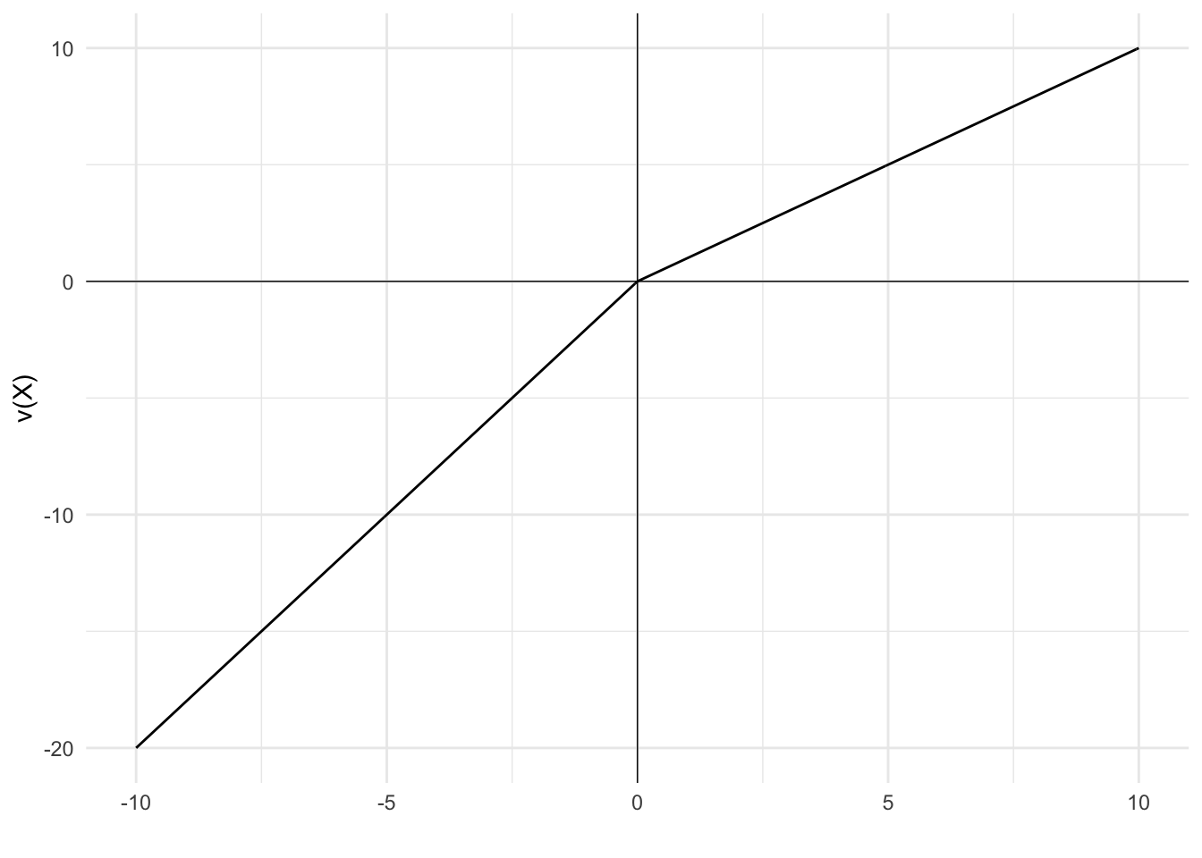
This plot shows the increased effect of the loss under this value function:
The greater slope of the curve in the loss domain, leading to a kink where the axes intercept, is indicative of the greater effect of losses.
13.3 The endowment effect
The endowment effect is often used to illustrate loss aversion.
Kahneman et al. (1991) ran one of the most famous and replicated experiments in economics.
They randomly assigned a free mug to members of a group and asked how much money they would accept for returning the mug (i.e. willingness to accept). The remaining participants were only shown a mug and asked about their willingness to pay for the mug.
Kahneman et al. (1991) found that the willingness to accept ($5.75) was substantially higher than the willingness to pay ($2.25).
The endowment effect is this phenomenon where people impute additional value to the items they own. The endowment effect is argued to be an empirical expression of loss aversion. Willingness to accept is higher as it is payment to incur the loss of the mug.
The endowment effect has been found in real estate markets, the stock market, with basketball tickets and in other domains.
13.3.1 Endowment effect example
Bruce has the following reference-dependent value function:
v(x)=\left\{\begin{matrix}
x \space &\textrm{where} \space x \geq 0\\
2x \space &\textrm{where} \space x<0
\end{matrix}\right.
x is the outcome relative to the reference point.
Assume Bruce has preferences over money (m) and mugs (c) as in this value function:
V(x)=v(m-r_m)+v(5c-5r_c)
r_m is Bruce’s reference point as it relates to money and r_c is his reference point as it relates to mugs.
To illustrate how this value function works, imagine Bruce has two mugs, and he drops one. It breaks. His change in the value function is:
At the beginning of the experiment, Bruce is given a mug. Assuming Bruce’s reference point adapts such that he considers the mug his, how much would Bruce need to be paid to give up the mug?
We can calculate this by calculating what payment \$p would make Bruce indifferent between losing the mug and gaining \$p. That is the point where, after losing the mug and receiving payment, Bruce’s change in value is equal to zero.
We assume a reference point for money of his current wealth and are instructed that his reference point for mugs is ownership of the mug.
Bruce would need to be paid at least $10 to give up the mug. Giving up the mug is seen as a loss and given greater weight than the money gained.
Now assume Bruce was not given a mug, but rather an opportunity to purchase a mug. How much would Bruce be willing to pay for the mug?
We can calculate this by calculating what payment $p would make Bruce indifferent between gaining the mug and losing $p. That is the point where, after receiving the mug and making payment, Bruce’s change in value is equal to zero.
We assume a reference point for money of his current wealth and are instructed that his reference point for mugs is no mug.
The most Bruce would be willing to pay for the mug is $2.50. He sees the foregone money as a loss, giving it greater weight than the mug gained.
Kahneman, D., Knetsch, J. L., and Thaler, R. H. (1991). Anomalies: The Endowment Effect, Loss Aversion, and Status Quo Bias. Journal of Economic Perspectives, 5(1), 193–206. https://doi.org/10.1257/jep.5.1.193