14 The reflection effect

Summary

The reflection effect is an asymmetry in risk preferences: people are typically risk-averse for gains but risk-seeking for losses.
This effect can be illustrated through framing experiments, such as the Asian Disease problem, where equivalent outcomes are perceived differently when framed as gains versus losses.
The reflection effect can be represented in a value function with diminishing sensitivity to both gains and losses, resulting in a concave function in the gain domain (indicating risk aversion) and a convex function in the loss domain (indicating risk-seeking behaviour).

14.1 Introduction

The reflection effect involves an asymmetry in risk preferences in the gain and loss domains.

When people make a risky choice related to gains, they are risk averse. They prefer a certain option with value lower than the expected value of the risky choice. When choosing an option in the loss domain, they become risk-seeking. This phenomenon is called the reflection effect.

Put simply, people typically prefer to lock in a sure gain rather than risk it for more, but will take risks to avoid a sure loss.

The reflection effect might also be thought of as diminishing sensitivity to gains or losses in either direction. This contrasts with expected utility theory, where the pain of losses increases as they grow in size.

14.2 The Asian Disease problem

The reflection effect explains the framing effects in the following experiment by Kahneman and Tversky (1984).

One group of experimental subjects were asked the following hypothetical question that would be unlikely to be asked post-Covid-19.

Imagine that the U.S. is preparing for the outbreak of an unusual Asian disease, which is expected to kill 600 people. Two alternative programs to combat the disease have been proposed. Assume that the exact scientific estimates of the consequences of the programs are as follows:

If Program A is adopted, 200 people will be saved.

If Program B is adopted, there is a one-third probability that 600 people will be saved and a two-thirds probability that no people will be saved.

Which of the two programs would you favour?

72% of participants chose option A.

Another group of experimental participants were shown the following:

Imagine that the U.S. is preparing for the outbreak of an unusual Asian disease, which is expected to kill 600 people. Two alternative programs to combat the disease have been proposed. Assume that the exact scientific estimates of the consequences of the programs are as follows:

If Program C is adopted, 400 people will die.

If Program D is adopted, there is a one-third probability that nobody will die and a two-thirds probability that 600 people will die.

Which of the two programs would you favour?

22% of participants chose option C.

Despite their differing presentation, these two scenarios are mathematically identical. Programs A and C both result in 200 people living and 400 dying. Similarly, Programs B and D offer a 1 in 3 chance of saving everyone and a 2 in 3 chance of everyone dying.

The difference is that the first scenario presents a ‘gain frame’, focusing on lives saved. The second scenario presents a ‘loss frame’, focusing on lives lost.” In the gain frame, 72% chose the certain option A over the risky option B. In the loss frame, only 22% chose the certain option C, meaning 78% preferred the risky option D.

This shift in preferences demonstrates the reflection effect. When the choice is framed in terms of gains - lives saved - people prefer the certain option. When framed in terms of losses - lives lost - they prefer the risky option.

14.3 The reflection effect in the value function

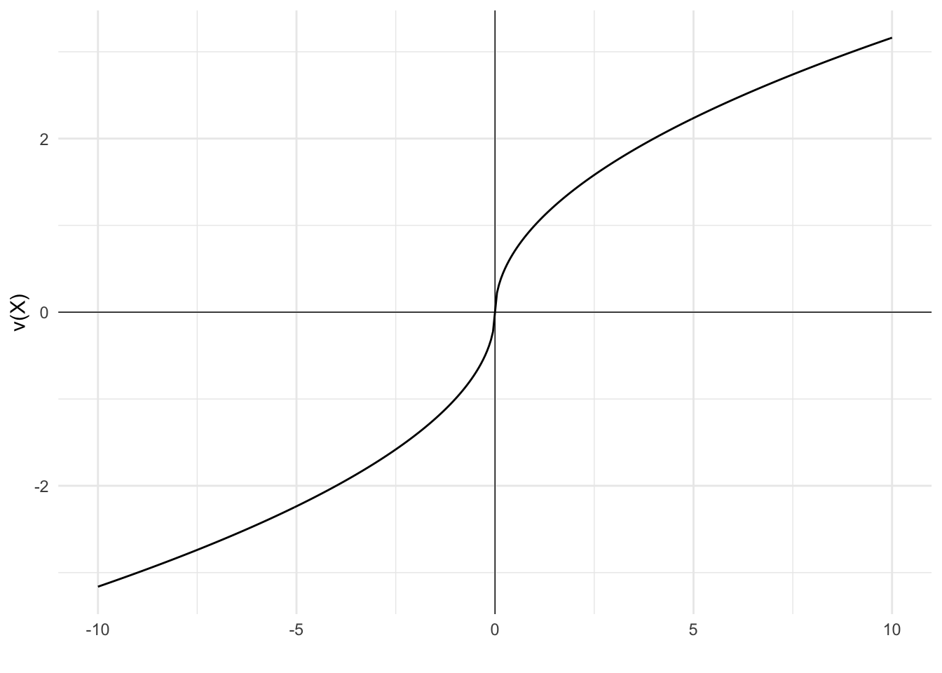
The following value function is an example of a function with diminishing sensitivity to both gains and losses. This function generates the reflection effect.

\begin{equation*} v(x)= \Bigg\{ \begin{matrix} x^\frac{1}{2} \space \text{where} \space x \geq 0\\ -(-x)^\frac{1}{2} \space \text{where} \space x<0 \end{matrix} \end{equation*}

As x increases in magnitude in either direction, the marginal change in value from each incremental unit of x decreases. This decreasing marginal change is implemented via the power of one half. For the value of the gain or loss to double, the size of the gain or loss must quadruple.

When x is less than zero, we apply a negative sign to x as the power of one half is only defined for positive numbers. We then apply another negative sign after applying the power to indicate the negative value of losses.

This value function results in risk-averse behaviour in the gain domain and risk-seeking behaviour in the loss domain. The following plot shows the diminishing effect in each direction.

Code

library(ggplot2)

loss_fun <- function(x){
  -(-x)^0.5
}
gain_fun <- function(x){
  x^0.5
}

loss <- data.frame(
  x=seq(-10,0,0.05),
  y=NA
  )
loss$y <- loss_fun(loss$x)

gain <- data.frame(
  x=seq(0,10,0.05),
  y=NA
  )
gain$y <- gain_fun(gain$x)

ggplot(mapping = aes(x, y)) +
  geom_line(data = loss) +
  geom_line(data = gain) + 
  geom_vline(xintercept = 0, linewidth=0.25)+ 
  geom_hline(yintercept = 0, linewidth=0.25)+
  labs(x = "x", y = "v(x)")+

  # Set the theme
  theme_minimal()+

  theme(axis.text.x = element_blank(),
            axis.text.y = element_blank(),
            axis.title=element_text(size=14,face="bold"),
            axis.title.y = element_text(angle=0, vjust=0.5))

In the gain domain, the function is concave, indicating risk aversion. In the loss domain, the convex function indicates risk-seeking behaviour. The result is an S-shaped curve.

14.4 An example

The following numerical example illustrates further.

Suppose an agent has a value function that expresses the reflection effect, with the outcomes in either direction subject to a power of one half.

\begin{equation*} v(x)= \Bigg\{ \begin{matrix} x^\frac{1}{2} \space \text{where} \space x \geq 0\\ -(-x)^\frac{1}{2} \space \text{where} \space x<0 \end{matrix} \end{equation*}

This agent is offered a choice between $10 for certain and a 50:50 bet to win $20 or end up with nothing. We calculate the value of each option by substituting the outcomes into the value function.

For the certain gain, we substitute $10 into the value function.

\begin{align*} v(\text{certainty})&=v(10) \\[6pt] &=10^{\frac{1}{2}} \\[6pt] &=3.16 \end{align*}

For the bet, we calculate the probability weighted value of the potential outcomes.

\begin{align*} v(\text{bet})&=0.5\times v(20)+0.5\times v(0) \\[6pt] &=0.5\times 20^{\frac{1}{2}}+0.5\times 0 \\[6pt] &=2.24 \end{align*}

The $10 for certain has a higher value for the agent. This agent is risk averse in the gain domain and therefore prefers an amount for certain over a bet with the same expected value.

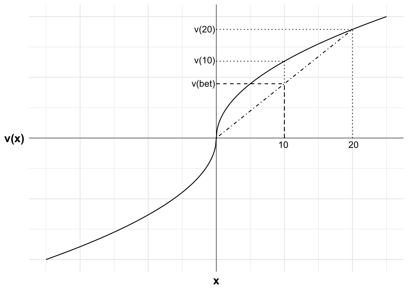
The following chart illustrates. Plotted are the value of the certain payment of $10 and the outcome from winning the gamble, $20. A loss results in value of 0.

The value of the gamble itself is the probability-weighted average of the two gamble outcomes. Due to diminishing marginal utility in the gain domain, the value of the gamble is less than the value of $10 with certainty. The extra $10 over the certain outcome from winning the bet is less than the value of the first $10. As a result, the agent does not want to risk the bet.

Code

library(ggplot2)

u <- function(x){
  ifelse (x >= 0, x^0.5, -(-x)^0.5)
}

df <- data.frame(
  x = seq(-25, 25, 0.1),
  y = u(seq(-25, 25, 0.1))
)

#Variables for plot (may not match labels as not done to scale)
#Payoffs from gamble
x1<-0 #loss
x2<-20 #win
ev<-10 #expected value of gamble
xc<-10 #certain outcome
px2<-(ev-x1)/(x2-x1)

ggplot(mapping = aes(x, y)) +

  #Plot the utility curve
  geom_line(data = df) +
  geom_vline(xintercept = 0, linewidth=0.25)+ 
  geom_hline(yintercept = 0, linewidth=0.25)+
  labs(x = "x", y = "v(x)")+

  # Set the theme
  theme_minimal()+

  #remove numbers on each axis
  theme(axis.text.x = element_blank(),
            axis.text.y = element_blank(),
            axis.title=element_text(size=14,face="bold"),
            axis.title.y = element_text(angle=0, vjust=0.5))+

  #limit to y greater than zero and x greater than -8 (need -8 so space for y-axis labels)
  coord_cartesian(xlim = c(-25, 25), ylim = c(-5, 5))+

  #Add labels 10, v(10) and line to curve indicating each
  annotate("text", x = xc, y = 0, label = "10", size = 4, hjust = 0.6, vjust = 1.5)+
  annotate("segment", x = xc, y = 0, xend = xc, yend = u(xc), linewidth = 0.5, colour = "black", linetype="dotted")+
  annotate("segment", x = 0, y = u(xc), xend = xc, yend = u(xc), linewidth = 0.5, colour = "black", linetype="dotted")+
  annotate("text", x = 0, y = u(xc), label = "v(10)", size = 4, hjust = 1.05, vjust = 0.3)+

  #Add expected utility line
  annotate("segment", x = x1, xend = x2, y = u(x1), yend = u(x2), linewidth = 0.5, colour = "black", linetype="dotdash")+

  #Add labels 20, v(20) and line to curve indicating each
  annotate("text", x = x2, y = 0, label = "20", size = 4, hjust = 0.4, vjust = 1.5)+
  annotate("segment", x = x2, y = 0, xend = x2, yend = u(x2), linewidth = 0.5, colour = "black", linetype="dotted")+
  annotate("segment", x = 0, y = u(x2), xend = x2, yend = u(x2), linewidth = 0.5, colour = "black", linetype="dotted")+
  annotate("text", x = 0, y = u(x2), label = "v(20)", size = 4, hjust = 1.05, vjust = 0.45)+

  #Add labels v(bet) and curve indicating position
  annotate("segment", x = ev, y = 0, xend = ev, yend = u(x1)+(u(x2)-u(x1))*px2, linewidth = 0.5, colour = "black", linetype="dashed")+
  annotate("segment", x = 0, y = u(x1)+(u(x2)-u(x1))*px2, xend = ev, yend = u(x1)+(u(x2)-u(x1))*px2, linewidth = 0.5, colour = "black", linetype="dashed")+
  annotate("text", x = 0, y = u(x1)+(u(x2)-u(x1))*px2, label = "v(bet)", size = 4, hjust = 1.05, vjust = 0.45)

Figure 14.2: The reflection effect in the gain domain

Suppose the agent is now offered another choice. They can now have a certain loss of $10 or a 50:50 bet to lose $20 or to lose nothing.

Again, we calculate the value of each option by substituting the outcomes into the value function.

For the certain loss, we substitute -$10 into the value function.

\begin{align*} v(\text{certainty})&=v(-10) \\[6pt] &=-10^{\frac{1}{2}} \\[6pt] &=-3.16 \end{align*}

For the bet, we calculate the probability weighted value of the potential outcomes.

\begin{align*} v(\text{bet})&=0.5\times v(-20)+0.5\times v(0) \\[6pt] &=-0.5\times 20^{\frac{1}{2}}+0.5\times 0 \\[6pt] &=-2.24 \end{align*}

This bet delivers higher value than the certain loss, despite the bet and the certain loss having the same expected value. The agent is willing to take a risk to avoid a loss. They are risk seeking in the loss domain.

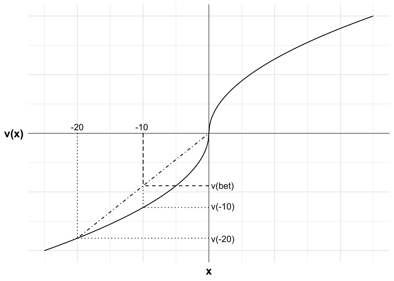
The following chart illustrates. Plotted are the value of the certain payment of -$10 and the outcome from losing the gamble, -$20. A win results in value of 0.

The value of the gamble itself is the probability-weighted average of the two gamble outcomes. Due to diminishing marginal utility in the loss domain, the value of the gamble is greater than the value of -$10 with certainty. The potential loss of another $10 over and above the certain loss is given less weight than the first $10. As a result, the agent wants to take the risk.

Code

library(ggplot2)

u <- function(x){
  ifelse (x >= 0, x^0.5, -(-x)^0.5)
}

df <- data.frame(
  x = seq(-25, 25, 0.1),
  y = u(seq(-25, 25, 0.1))
)

#Variables for plot (may not match labels as not done to scale)
#Payoffs from gamble
x1<--20 #loss
x2<-0 #win
ev<--10 #expected value of gamble
xc<--10 #certain outcome
px2<-(ev-x1)/(x2-x1)

ggplot(mapping = aes(x, y)) +

  #Plot the utility curve
  geom_line(data = df) +
  geom_vline(xintercept = 0, linewidth=0.25)+ 
  geom_hline(yintercept = 0, linewidth=0.25)+
  labs(x = "x", y = "v(x)")+

  # Set the theme
  theme_minimal()+

  #remove numbers on each axis
  theme(axis.text.x = element_blank(),
            axis.text.y = element_blank(),
            axis.title=element_text(size=14,face="bold"),
            axis.title.y = element_text(angle=0, vjust=0.5))+

  #limit to y greater than zero and x greater than -8 (need -8 so space for y-axis labels)
  coord_cartesian(xlim = c(-25, 25), ylim = c(-5, 5))+

  #Add labels -10, v(-10) and line to curve indicating each
  annotate("text", x = xc, y = 0, label = "-10", size = 4, hjust = 0.6, vjust = -0.5)+
  annotate("segment", x = xc, y = 0, xend = xc, yend = u(xc), linewidth = 0.5, colour = "black", linetype="dotted")+
  annotate("segment", x = 0, y = u(xc), xend = xc, yend = u(xc), linewidth = 0.5, colour = "black", linetype="dotted")+
  annotate("text", x = 0, y = u(xc), label = "v(-10)", size = 4, hjust = -0.1, vjust = 0.3)+

  #Add labels -20, v(-20) and line to curve indicating each
  annotate("text", x = x1, y = 0, label = "-20", size = 4, hjust = 0.5, vjust = -0.5)+
  annotate("segment", x = x1, y = 0, xend = x1, yend = u(x1), linewidth = 0.5, colour = "black", linetype="dotted")+
  annotate("segment", x = 0, y = u(x1), xend = x1, yend = u(x1), linewidth = 0.5, colour = "black", linetype="dotted")+
  annotate("text", x = 0, y = u(x1), label = "v(-20)", size = 4, hjust = -0.1, vjust = 0.6)+

  #Add expected utility line
  annotate("segment", x = x1, xend = x2, y = u(x1), yend = u(x2), linewidth = 0.5, colour = "black", linetype="dotdash")+

  #Add labels v(bet) and curve indicating position
  annotate("segment", x = ev, y = 0, xend = ev, yend = u(x1)+(u(x2)-u(x1))*px2, linewidth = 0.5, colour = "black", linetype="dashed")+
  annotate("segment", x = 0, y = u(x1)+(u(x2)-u(x1))*px2, xend = ev, yend = u(x1)+(u(x2)-u(x1))*px2, linewidth = 0.5, colour = "black", linetype="dashed")+
  annotate("text", x = 0, y = u(x1)+(u(x2)-u(x1))*px2, label = "v(bet)", size = 4, hjust = -0.1, vjust = 0.45)

Figure 14.3: The reflection effect in the loss domain