17 Probability weighting

In expected utility theory, probabilities enter the expected utility function linearly. For example, if an event is twice as likely as another outcome, it has double the weight.

In contrast, prospect theory incorporates non-linear weighting of probabilities by applying decision weights to each potential outcome.

17.1 Empirical evidence

Experimental observation indicates that we approximate linear weights for intermediate probabilities when making decisions under risk.

But, there is strong evidence that we overweight certain events, when the probability of the event is one, relative to near certain events, such as when the probability is, say, 99%. This overweighting of certainty is effectively the same as overweighting very low-probability events.

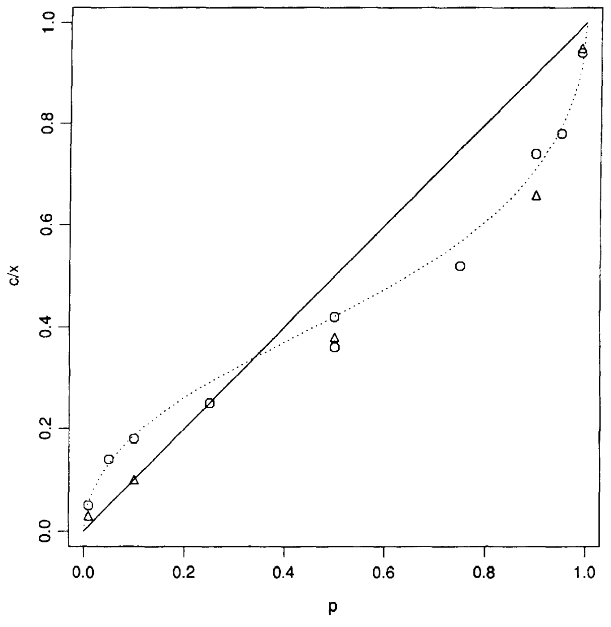
The following diagram from Tversky and Kahneman (1992) illustrates the relationship between objective probability and the decision weight applied to each outcome. On the x-axis is the probability of the outcome. On the y-axis is the weight applied to the value function for that probability. The straight line at 45 degrees represents linear weighting of probabilities. The curve represents the weighting function.

For this particular curve, where the probability is very low, such as around p=0.05, the weight is around 0.15. Similarly, at high probability, such as p=0.95, the weight is around 0.8. For intermediate probabilities, the observed weight is relatively closer to the objective probability.

Kahneman (2011) calls the large psychological value of the change from 0 to 5% (or some other small probability) the possibility effect. He calls the large psychological value of the change to 100% the certainty effect. We will pay a lot more for certainty than near certainty.

17.2 The Allais Paradox

Probability weighting is often offered as an explanation for the Allais Paradox, which I discuss in Section 11.1.

The Allais paradox can be illustrated as follows.

You are given the following pair of choices.

Choice 1: Choose one of the following bets:

Bet A:

$2500 with probability: 33%
$2400 with probability: 66%
$0 with probability: 1%

Bet B:

$2400 with probability: 100%

People tend to prefer Bet B.

Choice 2: Choose one of the following bets:

Bet C:

$2500 with probability: 33%
$0 with probability: 67%

Bet D:

$2400 with probability: 34%
$0 with probability: 66%

People tend to prefer Bet C.

It can be shown that this pair of preferences, Bet B and Bet C, does not conform with expected utility theory.

One explanation for this pair of decisions comes from probability weighting. If you look at Bet B, the outcome is certain. Certain events tend to be overweighted relative to near-certain events, such as the 99% chance of $2400 or $2500 in Bet A. An alternative way of thinking about this is that the 1% probability of nothing in Bet A is overweighted.

Conversely, the intermediate probabilities in Bet C and Bet D are weighted closer to linearly, which can result in the slightly higher expected value Bet C being preferred.

17.3 The decision weight

The weighting of probabilities is applied in prospect theory through a decision weight \pi(p_i). The decision weight is a function of the probability of the outcome.

This decision-weighting function reflects the empirical regularity that people overweight certain events relative to near-certain events and overweight low-probability events.

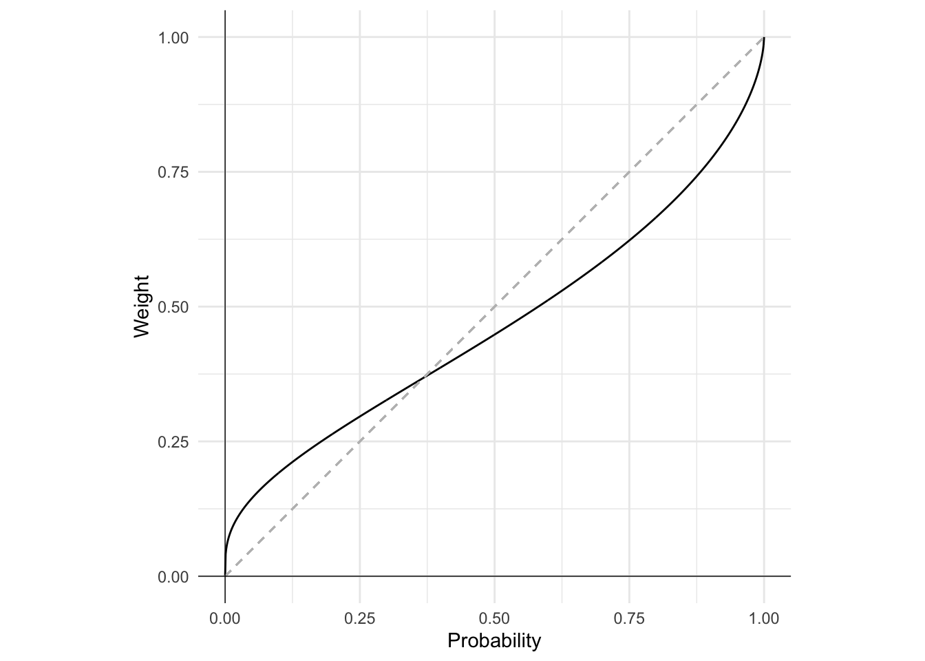
An example probability weighting function of a type proposed by Prelec (1998) is as follows:

\pi(p)=e^{-(-ln(p))^\alpha}\\[6pt] o<\alpha<1

This function, with \alpha=0.6, is plotted below.

Code

#Plot of probability weighting function using ggplot2
library(ggplot2)

#Define probability weighting function
prob_weight <- function(p, alpha){
  exp(-(-log(p))^alpha)
}

#Create data frame of probabilities and weights
prob <- seq(0, 1, 0.001)
prob_df <- data.frame(prob = prob, weight = prob_weight(prob, 0.6))

#Plot
ggplot(prob_df, aes(x = prob, y = weight)) +
  geom_line() +

  #Use geom_segment to add dashed light 45 degree line between 0 and 1
  geom_segment(x = 0, y = 0, xend = 1, yend = 1, linetype = "dashed", color = "grey") +

  #Add axes
  geom_vline(xintercept = 0, linewidth=0.25)+ 
  geom_hline(yintercept = 0, linewidth=0.25)+

  #Add labels
  labs(x = "Probability", y = "Weight") +

  #Make chart square
  coord_fixed()+

  #Set theme
  theme_minimal()

Figure 17.1: Probability weighting function