Code
equation <- function(W){
  log(W) - 0.6 * log(W + 100) - 0.4 * log(W - 100)
}

indifference <- uniroot(equation, c(200, 1000))Penny is an expected utility maximiser with utility function u(x)=\ln(x) and wealth of $300.
Penny is offered the following bet A:
a) Does Penny accept bet A?
Penny compares the utility of taking versus not taking the bet:
\begin{align*} U(\text{A})&=p_1u(x_1)+p_2u(x_2) \\ &=0.6\ln(W+150)+0.4\ln(W-100) \\ &=0.6\ln(450)+0.4\ln(200) \\ &=5.785 \\ \\ U(W)&=ln(W) \\ &=\ln(300) \\ &=5.704 \end{align*}
U(A)>U(W), so Penny accepts the bet.
b) Following some bad economic news, Penny wealth declines to $150.
Penny is offered bet A again. Does Penny accept the bet?
Penny compares the utility of taking versus not taking the bet:
\begin{align*} U(\text{A})&=p_1u(x_1)+p_2u(x_2) \\ &=0.6\ln(W+150)+0.4\ln(W-100) \\ &=0.6\ln(300)+0.4\ln(50) \\ &=4.987 \\ \\ U(W)&=\ln(W) \\ &=\ln(150) \\ &=5.011 \end{align*}
U(A)<U(W), so Penny rejects the bet.
Gamble A is as follows:
($100, 0.6; -$100, 0.4)
This is a gamble with a 60% chance of winning $100 and a 40% chance of losing $100.
a) Would a risk neutral decision-maker (who maximises expected value) be willing to pay $10 to play gamble A? What is the most they would be willing to pay to play?
A risk neutral decision maker will accept any offer with positive expected value. The expected value of the bet is:
\begin{align*} E[A]&=p_1x_1+p_2x_2 \\ &=0.6*100+0.4*(-100) \\ &=\$20 \end{align*}
The risk neutral decision maker would pay $10 as this is less than the expected value of the bet. They would be willing to pay up to the expected value of the bet: $20. At that point they would be indifferent between paying for the bet and refusing the bet.
b) Would an expected utility maximiser with wealth $200 and utility function U(x)=ln(x) be willing to pay $10 to play gamble A? What is the most they would be willing to pay to play?
The expected utility maximiser will play if their utility from playing and paying is greater than their utility of refusing.
\begin{align*} U(W)&=ln(W) \\ &=ln(\$200) \\ &=5.2983174 \\ \\ E[U(A-c)]&=p_1U(x_1)+p_2U(x_2) \\ &=0.6U(W+100-10)+0.4U(W-100-10) \\ &=0.6ln(200+100-10)+0.4ln(200-100-10) \\ &=5.2018524 \end{align*}
U(W)>U(A-c) so the decision maker will not be willing to pay $10.
To determine the most they would be willing to pay, we will first check whether they will pay any positive sum. We will do that by examining the expected utility of the gamble with no payment.
\begin{align*} E[U(A)]&=p_1U(x_1)+p_2U(x_2) \\ &=0.6U(W+100)+0.4U(W-100) \\ &=0.6ln(200+100)+0.4ln(200-100) \\ &=5.2643376 \end{align*}
U(W)>U() so the decision maker will not be willing to pay any amount. In fact, they would pay to avoid the bet.
To calculate how much, we determine what the certainty equivalent of the bet is:
\begin{align*} U(CE)&=E[U(A)] \\ ln(CE)&=5.2643376\\ CE&=e^{5.2643376} \\ &=\$ \end{align*}
Having wealth of $200 and the bet is the equivalent of having wealth of $193.32. They would be willing to pay up to $6.68 to avoid the bet.
c) Would the expected utility maximiser with utility function change their decision if they had $1000 in wealth? Explain.
The expected utility maximiser will play if their utility from playing and paying is greater than their utility of refusing.
\begin{align*} U(W)&=ln(W) \\ &=ln(\$1000) \\ &=6.9077553 \\ \\ E[U(A-c)]&=p_1U(x_1)+p_2U(x_2) \\ &=0.6U(W+100-10)+0.4U(W-100-10) \\ &=0.6ln(1000+100-10)+0.4ln(1000-100-10) \\ &=6.9128484 \end{align*}
U(W)<U(A-c) so the decision maker is now willing to pay $10.
As the agent’s wealth increases their utility function becomes increasingly linear (second derivative approaches zero) and they become closer to risk neutral. As a result, the positive expected value bet becomes increasingly attractive.
d) At what wealth is the expected utility maximiser with utility function U(x)=ln(x) indifferent between accepting gamble A or not?
The expected utility maximiser will be indifferent when:
\begin{align*} U(W)&=E[U(A)] \\ U(W)&=0.6U(W+100)+0.4U(W-100) \\ ln(W)&=0.6ln(W+100)+0.4ln(W-100) \end{align*}
There isn’t a simple closed form solution to this equation, but we know from questions b) and c) that W is somewhere between $200 and $1000.
If we wanted to calculate exact solution, you could use tool such as Mathematica or Matlab to solve, write a short code to solve in R or even iterate toward a solution using Excel.
equation <- function(W){
log(W) - 0.6 * log(W + 100) - 0.4 * log(W - 100)
}
indifference <- uniroot(equation, c(200, 1000))The expected utility maximiser is indifferent when W=$256.81.
Shannon and Simon are offered a choice between options A and B:
A: Lottery X=(0.5, -\$100; 0.5, -\$20). This is a gamble with a 50% chance of losing $100 and a 50% chance of losing $20.
B: A loss of $30 for certain.
(a) Shannon is risk-neutral. Will Shannon choose A or B?
A risk-neutral decision-maker maximises expected value.
The expected value of option A is:
\begin{align*} \text{E}[A]&=p_1x_1+p_2x_2 \\[6pt] &=0.5\times -\$100+0.5\times -\$20 \\[6pt] &=-\$60 \end{align*}
The expected value of option B is -$30.
Shannon will choose the certain loss because -$30 is a better outcome than -$60.
(b) Simon is risk averse with wealth $200 and utility function U(x)=x^{0.5}. Will Simon choose A or B?
Simon will select the option that gives the highest expected utility.
The expected utility of option A is:
\begin{align*} \text{E}[U(A)]&=p_1u(x_1)+p_2u(x_2) \\[6pt] &=0.5\times (W-100)^{0.5}+0.5\times (W-20)^{0.5} \\[6pt] &=0.5\times (100)^{0.5}+0.5\times (180)^{0.5} \\[6pt] &=11.71 \end{align*}
The expected utility of option B is:
\begin{align*} \text{E}[U(B)]&=u(W+x) \\[6pt] &=(200-30)^{0.5} \\[6pt] &=13.04 \end{align*}
Simon will choose option B because \text{E}[U(A)]=11.71<13.04=\text{E}[U(B)].
(c) Draw a graph showing the choices faced by Simon, his utility curve and the expected utility of each option. Indicate the certainty equivalent of option A. Explain how the graph shows which option Simon will choose.
This chart shows the choices faced by Simon, his utility curve and the expected utility of each option. The horizontal axis is the outcome and the vertical axis is utility of each outcome. The utility curve is the function U(x)=x^{0.5}.
The two possible outcomes of gamble A are W-100=100 and W-20=180, which deliver U(W-100) and U(W-20) respectively. Each are labelled on the chart.
The expected utility of gamble A is the weighted average of these two utilities and lies on the straight line between U(W-100) and U(W-20). As each outcome has a 50% chance of occurring, the expected utility of gamble A is the midpoint of this line (as is the expected value of the gamble). The vertical line from W+E[A]=140 identifies that point, with the expected utility E[U(A)] marked on the vertical axis.
The certain outcome from option B, the loss of $30 resulting in wealth of $170 is also marked on the x-axis, leading to utility of U(W-B).
It can be seen that the expected utility of gamble A, E[U(A)], is less than the utility of the certain outcome U(W-B). Simon will therefore choose B.
The certainty equivalent of option A is identified as the point where U(CE)=E[U(A)]. This is identified by drawing a horizontal line from the expected utility of gamble A to the utility curve. The point where this line intersects the utility curve is the certainty equivalent of gamble A, shown by projecting a vertical line downward.
This diagram is not drawn to scale.
library(ggplot2)

u <- function(x){
  x^0.5
}

df <- data.frame(
  x=seq(0,220,0.1),
  y=NA
)

df$y <- u(df$x)

#Variables for plot (may not match labels as not done to scale)
#Payoffs from gamble
x1<-30 #loss
x2<-200 #win
ev<-115 #expected value of gamble
xc<-140 #certain outcome
ce<-95 #certainty equivalent
px2<-(ev-x1)/(x2-x1)

ggplot(mapping = aes(x, y)) +

  #Plot the utility curve
  geom_line(data = df) +
  geom_vline(xintercept = 0, linewidth=0.25)+
  geom_hline(yintercept = 0, linewidth=0.25)+
  labs(x = "x", y = "U(x)")+

  # Set the theme
  theme_minimal()+

  #remove numbers on each axis
  theme(axis.text.x = element_blank(),
            axis.text.y = element_blank(),
            axis.title=element_text(size=14,face="bold"),
            axis.title.y = element_text(angle=0, vjust=0.5))+

  #limit to y greater than zero and x greater than -8 (need -8 so space for y-axis labels)
  coord_cartesian(xlim = c(-25, 220), ylim = c(0,15))+

  #Add labels W-100, U(W-100) and line to curve indicating each
  annotate("text", x = x1, y = 0, label = "W-100", size = 4, hjust = 0.5, vjust = 1.5)+
  annotate("segment", x = x1, y = 0, xend = x1, yend = u(x1), linewidth = 0.5, colour = "black", linetype="dotted")+
  annotate("segment", x = 0, y = u(x1), xend = x1, yend = u(x1), linewidth = 0.5, colour = "black", linetype="dotted")+
  annotate("text", x = 0, y = u(x1), label = "U(W-100)", size = 4, hjust = 1.05, vjust = 0.6)+

  #Add labels W-B, U(W-B) and line to curve indicating each
  annotate("text", x = xc, y = 0, label = "W-B", size = 4, hjust = 0.6, vjust = 1.5)+
  annotate("segment", x = xc, y = 0, xend = xc, yend = u(xc), linewidth = 0.5, colour = "black", linetype="dotted")+
  annotate("segment", x = 0, y = u(xc), xend = xc, yend = u(xc), linewidth = 0.5, colour = "black", linetype="dotted")+
  annotate("text", x = 0, y = u(xc), label = "U(W-B)", size = 4, hjust = 1.05, vjust = 0.3)+

  #Add expected utility line
  annotate("segment", x = x1, xend = x2, y = u(x1), yend = u(x2), linewidth = 0.5, colour = "black", linetype="dotdash")+

  #Add labels W-20, U(W-20) and line to curve indicating each
  annotate("text", x = x2, y = 0, label = "W-20", size = 4, hjust = 0.4, vjust = 1.5)+
  annotate("segment", x = x2, y = 0, xend = x2, yend = u(x2), linewidth = 0.5, colour = "black", linetype="dotted")+
  annotate("segment", x = 0, y = u(x2), xend = x2, yend = u(x2), linewidth = 0.5, colour = "black", linetype="dotted")+
  annotate("text", x = 0, y = u(x2), label = "U(W-20)", size = 4, hjust = 1.05, vjust = 0.45)+

  #Add labels W+E[A], E[U(W+A)] and curve indicating each
  annotate("text", x = ev, y = 0, label = "W+E[A]", size = 4, hjust = 0.4, vjust = 1.5)+
  annotate("segment", x = ev, y = 0, xend = ev, yend = u(x1)+(u(x2)-u(x1))*px2, linewidth = 0.5, colour = "black", linetype="dashed")+
  annotate("segment", x = 0, y = u(x1)+(u(x2)-u(x1))*px2, xend = ev, yend = u(x1)+(u(x2)-u(x1))*px2, linewidth = 0.5, colour = "black", linetype="dashed")+
  annotate("text", x = 0, y = u(x1)+(u(x2)-u(x1))*px2, label = "E[U(A)]", size = 4, hjust = 1.05, vjust = 0.45)+

  #Add vertical line indicating certainty equivalent and labelled "CE"
  annotate("segment", x = ce, xend = ce, y = 0, yend = u(ce), linewidth = 0.5, colour = "black", linetype="dotted")+
  annotate("text", x = ce, y = 0, label = "CE", size = 4, hjust = 0.4, vjust = 1.5)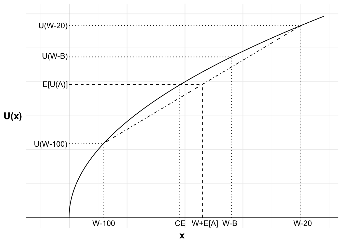
(a) Stacey, an expected utility maximiser, was considering quitting her job to start a new business. She calculated that her business proposal had a positive expected value but that there is a material risk of a loss. She decided not to start the business.
Use concepts from expected utility theory to explain why Stacey may have decided not to start the business.
Stacey may have decided not to pursue the business opportunity as she is risk averse. Someone who is risk averse will value the expected value of a gamble less than the equivalent amount paid with certainty. This means that a positive value bet might be turned down.
(b) Use a graph to demonstrate your answer to part (a).
This graph shows Stavey’s utility curve. As she is risk averse, the curve is concave (at least over the domain of the decisions we are considering).
Suppose there are two possible outcomes from starting the business. a moderate loss and a large gain, each having equal probability. Each of the outcomes of the business are labelled. Stacey finishes with his wealth minus the business loss (W-L) or her wealth plus the business gains (W+G). If she does not start the business, her wealth remains at W. The utility of each possible outcome (U(W-L), U(W), U(W+G)) is also indicated on the vertical axis.
The expected value of starting the business is labelled (E[X]). As the business has positive expected value, E[X] is greater than W.
The expected utility of the business lies on the straight line between the utility of the two possible business outcomes. The place on the line is determined by the probability of winning and is in line with the expected value of the business. We can identify the expected utility of the business by projecting a line up from E[X] to the straight line.
Finally, the certainty equivalent of the business is also marked. As U(CE)=E[U(X)], we can identify the certainty equivalent by projecting a line up from E[U(X)] to the utility curve.
Due to the convex curve, we can see that E[U(X)] is less than U(W). Stacey prefers the certain outcome of W to starting the business. Alternatively, we can see that the certainty equivalent of the business is lower than current wealth.
#| fig-cap: Stacey's consideration of whether to purchase a business ticket

library(ggplot2)

u <- function(x){
  x^0.5
}

df <- data.frame(
  x=seq(1,220,0.1),
  y=NA
)

df$y <- u(df$x)

#Variables for plot (may not match labels as not done to scale)
#Payoffs from gamble
x1<-30 #loss
x2<-200 #win
ev<-90 #expected value of gamble
xc<-80 #certain outcome
ce<-70 #certainty equivalent
px2<-(ev-x1)/(x2-x1)

ggplot(mapping = aes(x, y)) +

  #Plot the utility curve
  geom_line(data = df) +
  geom_vline(xintercept = 0, linewidth=0.25)+
  geom_hline(yintercept = 0, linewidth=0.25)+
  labs(x = "x", y = "U(x)")+

  # Set the theme
  theme_minimal()+

  #remove numbers on each axis
  theme(axis.text.x = element_blank(),
            axis.text.y = element_blank(),
            axis.title=element_text(size=14,face="bold"),
            axis.title.y = element_text(angle=0, vjust=0.5))+

  #limit to y greater than zero and x greater than -8 (need -8 so space for y-axis labels)
  coord_cartesian(xlim = c(-25, 220), ylim = c(0, 15))+

  #Add labels W-L, U(W-L) and line to curve indicating each
  annotate("text", x = x1, y = 0, label = "W-L", size = 4, hjust = 0.5, vjust = 1.5)+
  annotate("segment", x = x1, y = 0, xend = x1, yend = u(x1), linewidth = 0.5, colour = "black", linetype="dotted")+
  annotate("segment", x = 0, y = u(x1), xend = x1, yend = u(x1), linewidth = 0.5, colour = "black", linetype="dotted")+
  annotate("text", x = 0, y = u(x1), label = "U(W-L)", size = 4, hjust = 1.05, vjust = 0.6)+

  #Add labels W, U(W) and line to curve indicating each
  annotate("text", x = xc, y = 0, label = "W", size = 4, hjust = 0.6, vjust = 1.5)+
  annotate("segment", x = xc, y = 0, xend = xc, yend = u(xc), linewidth = 0.5, colour = "black", linetype="dotted")+
  annotate("segment", x = 0, y = u(xc), xend = xc, yend = u(xc), linewidth = 0.5, colour = "black", linetype="dotted")+
  annotate("text", x = 0, y = u(xc), label = "U(W)", size = 4, hjust = 1.05, vjust = 0.3)+

  #Add expected utility line
  annotate("segment", x = x1, xend = x2, y = u(x1), yend = u(x2), linewidth = 0.5, colour = "black", linetype="dotdash")+

  #Add labels W+G, U(W+G) and line to curve indicating each
  annotate("text", x = x2, y = 0, label = "W+G", size = 4, hjust = 0.4, vjust = 1.5)+
  annotate("segment", x = x2, y = 0, xend = x2, yend = u(x2), linewidth = 0.5, colour = "black", linetype="dotted")+
  annotate("segment", x = 0, y = u(x2), xend = x2, yend = u(x2), linewidth = 0.5, colour = "black", linetype="dotted")+
  annotate("text", x = 0, y = u(x2), label = "U(W+G)", size = 4, hjust = 1.05, vjust = 0.45)+

  #Add labels E[X], E[U(X)] and curve indicating each
  annotate("text", x = ev, y = 0, label = "E[X]", size = 4, hjust = 0.4, vjust = 1.5)+
  annotate("segment", x = ev, y = 0, xend = ev, yend = u(x1)+(u(x2)-u(x1))*px2, linewidth = 0.5, colour = "black", linetype="dashed")+
  annotate("segment", x = 0, y = u(x1)+(u(x2)-u(x1))*px2, xend = ev, yend = u(x1)+(u(x2)-u(x1))*px2, linewidth = 0.5, colour = "black", linetype="dashed")+
  annotate("text", x = 0, y = u(x1)+(u(x2)-u(x1))*px2, label = "E[U(X)]", size = 4, hjust = 1.05, vjust = 0.45)+

  #Add vertical line indicating certainty equivalent and labelled "CE"
  annotate("segment", x = ce, xend = ce, y = 0, yend = u(ce), linewidth = 0.5, colour = "black", linetype="dotted")+
  annotate("text", x = ce, y = 0, label = "CE", size = 4, hjust = 0.4, vjust = 1.5)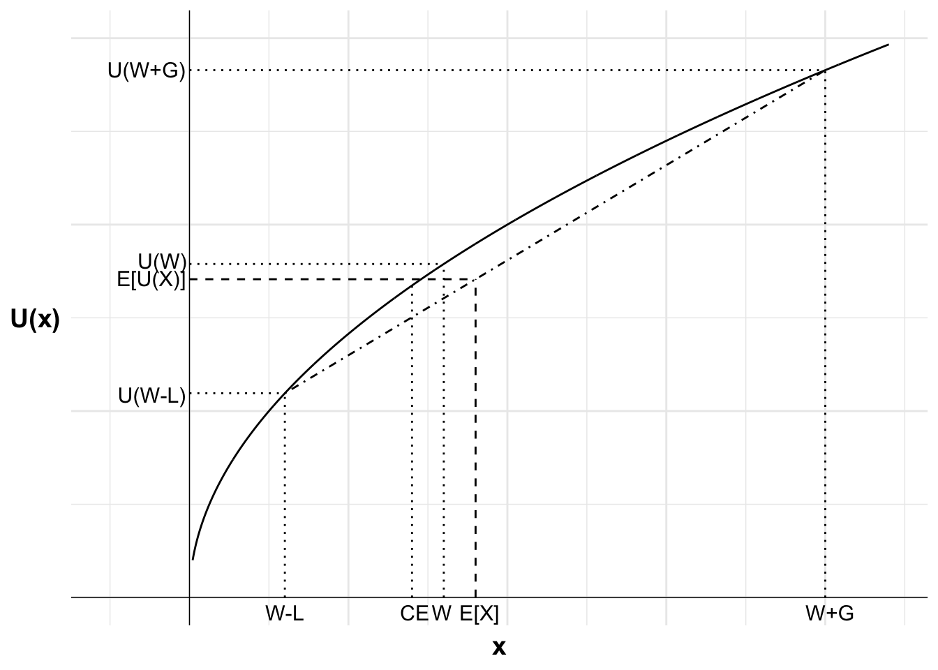
(c) Later, Stacey received a large inheritance from her Aunt. She then decided to quit work and go ahead with her business plan.
Use concepts from expected utility theory to explain why Stacey may have changed her mind.
That Stacey later decided to pursue the business opportunity is likely because she is more risk neutral (or possibly even risk seeking) at higher wealth. The result is that the positive expected value gamble is more likely to be accepted at the higher wealth level.
One mechanism by which this could occur is the utility function becomes increasingly linear with higher wealth (as is the case with u(x)=\ln(x) or u(x)=x^{0.5}).
Anika and Anthony are offered a choice between options A and B:
A: Lottery A=(0.5, \$100; 0.5, \$20). This is a gamble with a 50% chance of winning $100 and a 50% chance of winning $20.
B: $40 for certain.
(a) Anika is risk-neutral. Will Anika choose A or B?
A risk-neutral decision-maker maximises expected value.
The expected value of option A is:
\begin{align*} \text{E}[A]&=p_1x_1+p_2x_2 \\[6pt] &=0.5\times \$100+0.5\times \$20 \\[6pt] &=\$60 \end{align*}
The expected value of option B is $40.
Anika will choose option A because $60 is greater than $40.
(b) Anthony is risk averse with wealth $100 and utility function U(x)=\text{ln}(x). Will Anthony choose A or B?
Anthony will select the option that gives the highest expected utility.
The expected utility of option A is:
\begin{align*} \text{E}[U(A)]&=p_1u(x_1)+p_2u(x_2) \\[6pt] &=0.5\times \text{ln}(W+100)+0.5\times \text{ln}(W+20) \\[6pt] &=0.5\times \text{ln}(200)+0.5\times \text{ln}(120) \\[6pt] &=5.04 \end{align*}
The expected utility of option B is:
\begin{align*} \text{E}[U(B)]&=u(W+x) \\[6pt] &=\text{ln}(140) \\[6pt] &=4.94 \end{align*}
Anthony will choose option A because \text{E}[U(A)]=5.04>4.94=\text{E}[U(B)].
(c) Draw a graph showing the choices faced by Anthony, his utility curve and the expected utility of each option. Indicate the certainty equivalent of option A. Explain how the graph shows which option Anthony will choose.
Figure 53.1 shows the choices faced by Anthony, his utility curve and the expected utility of each option. The horizontal axis is the outcome and the vertical axis is utility of each outcome. The utility curve is the function U(x)=\text{ln}(x).
The two possible outcomes of gamble A are W+20=120 and W+100=200, which deliver U(W+20) and U(W+100) respectively. Each are labelled on the chart.
The expected utility of gamble A is the weighted average of these two utilities and lies on the straight line between U(W+20) and U(W+100). As each outcome has a 50% chance of occurring, the expected utility of gamble A is the midpoint of this line (as is the expected value of the gamble). The vertical line from W+E[A]=160 identifies that point, with the expected utility E[U(A)] marked on the vertical axis.
The certain outcome from option B, the receipt of $40 resulting in wealth of $140 is also marked on the x-axis, leading to utility of U(W+B).
It can be seen that the expected utility of gamble A E[U(A)] is greater than the utility of the certain outcome U(W+B). Anthony will therefore choose gamble A.
The certainty equivalent of option A is identified as the point where U(CE)=E[U(A)]. This is identified by drawing a horizontal line from the expected utility of gamble A to the utility curve. The point where this line intersects the utility curve is the certainty equivalent of gamble A, shown by projecting a vertical line downward.
This diagram is not drawn to scale.
library(ggplot2)

u <- function(x){
  log(x)
}

df <- data.frame(
  x=seq(1,220,0.1),
  y=NA
)

df$y <- u(df$x)

#Variables for plot (may not match labels as not done to scale)
#Payoffs from gamble
x1<-30 #loss
x2<-200 #win
ev<-115 #expected value of gamble
xc<-60 #certain outcome
ce<-79 #certainty equivalent
px2<-(ev-x1)/(x2-x1)

ggplot(mapping = aes(x, y)) +

  #Plot the utility curve
  geom_line(data = df) +
  geom_vline(xintercept = 0, linewidth=0.25)+
  geom_hline(yintercept = 0, linewidth=0.25)+
  labs(x = "x", y = "U(x)")+

  # Set the theme
  theme_minimal()+

  #remove numbers on each axis
  theme(axis.text.x = element_blank(),
            axis.text.y = element_blank(),
            axis.title=element_text(size=14,face="bold"),
            axis.title.y = element_text(angle=0, vjust=0.5))+

#set limits - need to include room for labels
  coord_cartesian(xlim = c(-25, 220), ylim = c(-0.25, 6))+

  #Add labels W+20, U(W+20) and line to curve indicating each
  annotate("text", x = x1, y = 0, label = "W+20", size = 4, hjust = 0.5, vjust = 1.5)+
  annotate("segment", x = x1, y = 0, xend = x1, yend = u(x1), linewidth = 0.5, colour = "black", linetype="dotted")+
  annotate("segment", x = 0, y = u(x1), xend = x1, yend = u(x1), linewidth = 0.5, colour = "black", linetype="dotted")+
  annotate("text", x = 0, y = u(x1), label = "U(W+20)", size = 4, hjust = 1.05, vjust = 0.6)+

  #Add labels W+B, U(W+B) and line to curve indicating each
  annotate("text", x = xc, y = 0, label = "W+B=140", size = 4, hjust = 0.6, vjust = 1.5)+
  annotate("segment", x = xc, y = 0, xend = xc, yend = u(xc), linewidth = 0.5, colour = "black", linetype="dotted")+
  annotate("segment", x = 0, y = u(xc), xend = xc, yend = u(xc), linewidth = 0.5, colour = "black", linetype="dotted")+
  annotate("text", x = 0, y = u(xc), label = "U(W+B)", size = 4, hjust = 1.05, vjust = 0.3)+

  #Add expected utility line
  annotate("segment", x = x1, xend = x2, y = u(x1), yend = u(x2), linewidth = 0.5, colour = "black", linetype="dotdash")+

  #Add labels W+100, U(W+100) and line to curve indicating each
  annotate("text", x = x2, y = 0, label = "W+100", size = 4, hjust = 0.4, vjust = 1.5)+
  annotate("segment", x = x2, y = 0, xend = x2, yend = u(x2), linewidth = 0.5, colour = "black", linetype="dotted")+
  annotate("segment", x = 0, y = u(x2), xend = x2, yend = u(x2), linewidth = 0.5, colour = "black", linetype="dotted")+
  annotate("text", x = 0, y = u(x2), label = "U(W+100)", size = 4, hjust = 1.05, vjust = 0.45)+

  #Add labels W+E[A], E[U(W+A)] and curve indicating each
  annotate("text", x = ev, y = 0, label = "W+E[A]=160", size = 4, hjust = 0.4, vjust = 1.5)+
  annotate("segment", x = ev, y = 0, xend = ev, yend = u(x1)+(u(x2)-u(x1))*px2, linewidth = 0.5, colour = "black", linetype="dashed")+
  annotate("segment", x = 0, y = u(x1)+(u(x2)-u(x1))*px2, xend = ev, yend = u(x1)+(u(x2)-u(x1))*px2, linewidth = 0.5, colour = "black", linetype="dashed")+
  annotate("text", x = 0, y = u(x1)+(u(x2)-u(x1))*px2, label = "E[U(A)]", size = 4, hjust = 1.05, vjust = 0.45)+

  #Add vertical line indicating certainty equivalent and labelled "CE"
  annotate("segment", x = ce, xend = ce, y = 0, yend = u(ce), linewidth = 0.5, colour = "black", linetype="dotted")+
  annotate("text", x = ce, y = 0, label = "CE", size = 4, hjust = 0.4, vjust = 1.5)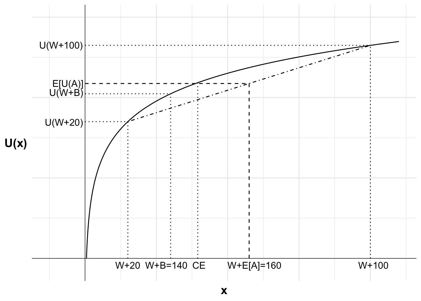
Buying a lottery ticket has a negative expected value. Andrew is an expected utility maximiser. He purchases a lottery ticket.
(a) What risk preferences (attitude to risk) does Andrew have?
If an expected utility maximiser purchases a lottery ticket with negative expected value, he is risk seeking. He values the gamble over and above the expected value of the gamble.
(b) Use a graph to demonstrate your answer to part (a).
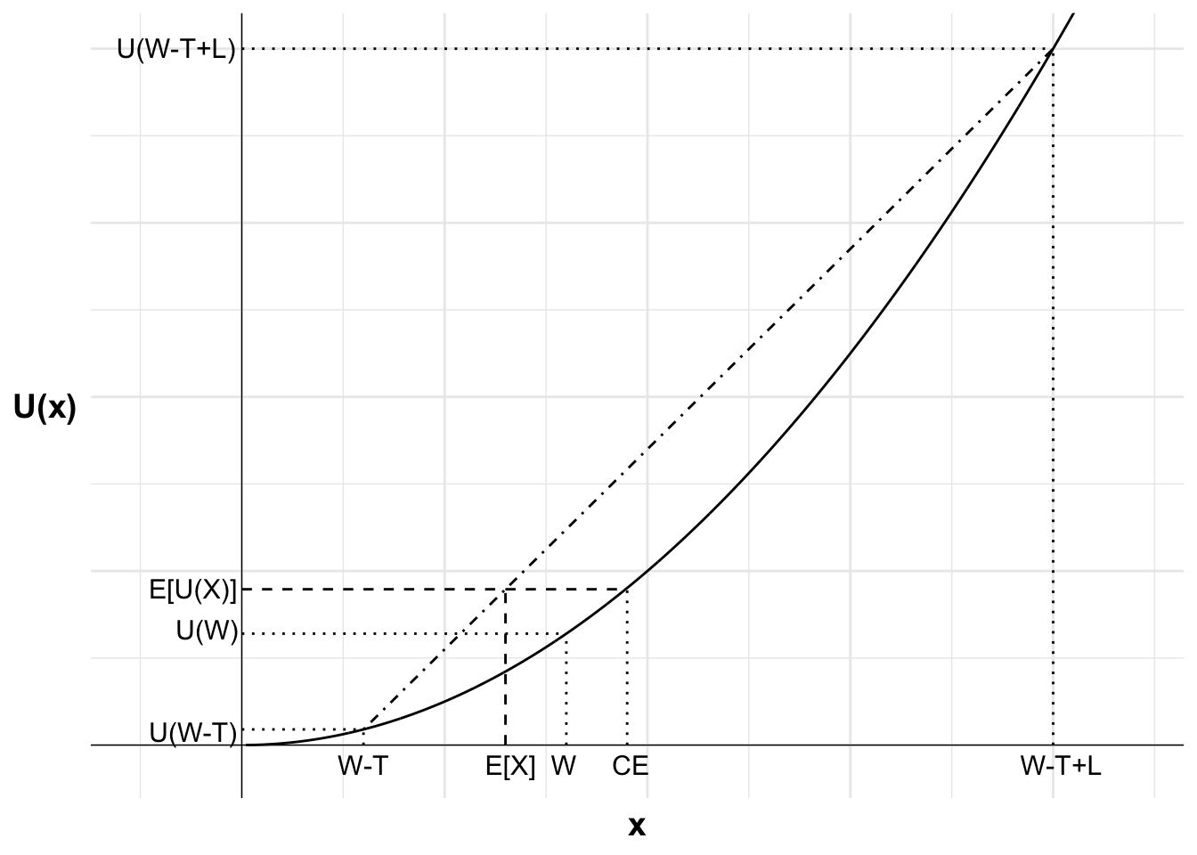
Figure 53.2 shows Andrew’s utility curve. As he is risk seeking it is convex (at least over the domain of the lottery).
Each of the outcomes of the lottery are labelled. Andrew finishes with his wealth minus the cost of the lottery ticket (W-T) or his wealth minus the cost of the lottery ticket plus his lottery winnings (W-T+L). If he does not purchase the ticket, his wealth remains at W. The utility of each possible outcome (U(W-T), U(W), U(W-T+L)) is also indicated on the vertical axis.
The expected value of the lottery after buying the ticket is labelled (E[X]). As the lottery has a negative expected value, E[X] is less than W.
The expected utility of the lottery lies on the straight line between the utility of the two possible lottery outcomes. The place on the line is determined by the probability of winning and is in line with the expected value of the lottery. We can identify the expected utility of the lottery by projecting a line up from E[X] to the straight line.
Finally, the certainty equivalent of the lottery is also marked. As U(CE)=E[U(X)], we can identify the certainty equivalent by projecting a line up from E[U(X)] to the utility curve.
Due to the convex curve, we can see that E[U(X)] is greater than U(W). Andrew prefers the lottery to the certain outcome of W. Alternatively, we can see that the certainty equivalent of the lottery is higher than current wealth. Andrew would require a payment of at least CE-W to forgo his opportunity to partake in the lottery.
library(ggplot2)

u <- function(x){
  x^2
}

df <- data.frame(
  x=seq(1,220,0.1),
  y=NA
)

df$y <- u(df$x)

#Variables for plot (may not match labels as not done to scale)
#Payoffs from gamble
x1<-30 #loss
x2<-200 #win
ev<-65 #expected value of gamble
xc<-80 #certain outcome
ce<-95 #certainty equivalent
px2<-(ev-x1)/(x2-x1)

ggplot(mapping = aes(x, y)) +

  #Plot the utility curve
  geom_line(data = df) +
  geom_vline(xintercept = 0, linewidth=0.25)+
  geom_hline(yintercept = 0, linewidth=0.25)+
  labs(x = "x", y = "U(x)")+

  # Set the theme
  theme_minimal()+

  #remove numbers on each axis
  theme(axis.text.x = element_blank(),
            axis.text.y = element_blank(),
            axis.title=element_text(size=14,face="bold"),
            axis.title.y = element_text(angle=0, vjust=0.5))+

#set limits - need to include room for labels
  coord_cartesian(xlim = c(-25, 220), ylim = c(-1000, 40000))+

  #Add labels W-T, U(W-T) and line to curve indicating each
  annotate("text", x = x1, y = 0, label = "W-T", size = 4, hjust = 0.5, vjust = 1.5)+
  annotate("segment", x = x1, y = 0, xend = x1, yend = u(x1), linewidth = 0.5, colour = "black", linetype="dotted")+
  annotate("segment", x = 0, y = u(x1), xend = x1, yend = u(x1), linewidth = 0.5, colour = "black", linetype="dotted")+
  annotate("text", x = 0, y = u(x1), label = "U(W-T)", size = 4, hjust = 1.05, vjust = 0.6)+

  #Add labels W, U(W) and line to curve indicating each
  annotate("text", x = xc, y = 0, label = "W", size = 4, hjust = 0.6, vjust = 1.5)+
  annotate("segment", x = xc, y = 0, xend = xc, yend = u(xc), linewidth = 0.5, colour = "black", linetype="dotted")+
  annotate("segment", x = 0, y = u(xc), xend = xc, yend = u(xc), linewidth = 0.5, colour = "black", linetype="dotted")+
  annotate("text", x = 0, y = u(xc), label = "U(W)", size = 4, hjust = 1.05, vjust = 0.3)+

  #Add expected utility line
  annotate("segment", x = x1, xend = x2, y = u(x1), yend = u(x2), linewidth = 0.5, colour = "black", linetype="dotdash")+

  #Add labels W-T+L, U(W-T+L) and line to curve indicating each
  annotate("text", x = x2, y = 0, label = "W-T+L", size = 4, hjust = 0.4, vjust = 1.5)+
  annotate("segment", x = x2, y = 0, xend = x2, yend = u(x2), linewidth = 0.5, colour = "black", linetype="dotted")+
  annotate("segment", x = 0, y = u(x2), xend = x2, yend = u(x2), linewidth = 0.5, colour = "black", linetype="dotted")+
  annotate("text", x = 0, y = u(x2), label = "U(W-T+L)", size = 4, hjust = 1.05, vjust = 0.45)+

  #Add labels E[X], E[U(X)] and curve indicating each
  annotate("text", x = ev, y = 0, label = "E[X]", size = 4, hjust = 0.4, vjust = 1.5)+
  annotate("segment", x = ev, y = 0, xend = ev, yend = u(x1)+(u(x2)-u(x1))*px2, linewidth = 0.5, colour = "black", linetype="dashed")+
  annotate("segment", x = 0, y = u(x1)+(u(x2)-u(x1))*px2, xend = ev, yend = u(x1)+(u(x2)-u(x1))*px2, linewidth = 0.5, colour = "black", linetype="dashed")+
  annotate("text", x = 0, y = u(x1)+(u(x2)-u(x1))*px2, label = "E[U(X)]", size = 4, hjust = 1.05, vjust = 0.45)+

  #Add vertical line indicating certainty equivalent and labelled "CE"
  annotate("segment", x = ce, xend = ce, y = 0, yend = u(ce), linewidth = 0.5, colour = "black", linetype="dotted")+
  annotate("segment", x = ev, y = u(x1)+(u(x2)-u(x1))*px2, xend = ce, yend = u(x1)+(u(x2)-u(x1))*px2, linewidth = 0.5, colour = "black", linetype="dashed")+
  annotate("text", x = ce, y = 0, label = "CE", size = 4, hjust = 0.4, vjust = 1.5)