Prospect theory can explain various real-world economic behaviours that deviate from traditional economic models, as illustrated by studies on taxi drivers, investors, and homeowners.
Some studies on taxi driver behaviour on rainy days suggest that drivers may have a daily earnings target (reference point), and their decisions reflect loss aversion and diminishing sensitivity to gains, key elements of prospect theory.
The disposition effect in investing, where investors tend to sell winning stocks and hold losing ones, can be explained by prospect theory’s reflection effect.
In the housing market, owners subject to nominal losses tend to set higher asking prices, potentially due to loss aversion.
However, follow-up studies and alternative explanations demonstrate that the application of prospect theory to these scenarios is not without controversy, and results can vary based on methodology and data interpretation.
19.1 Introduction
In this part, I discuss some applied problems that have been analysed using prospect theory.
19.2 Taxi driver behaviour on rainy days
Why can’t you find a taxi on a rainy day?
One possible explanation comes from Colin Camerer et al. (1997), who studied the labour supply of New York City taxi drivers.
The taxi drivers rent a cab for a 12-hour period for a fixed fee, plus petrol. Within the 12 hours, a driver can choose how long they keep the taxi out.
A taxi driver’s effective wage can vary for many reasons, such as weather, subway breakdowns, day of the week and conferences. When they are busier, they have a higher effective wage. That is, they earn more fares.
In two of the three samples they examined, Camerer et al. found that drivers drove less when their effective wages were higher. This was the case for inexperienced drivers in all three samples, and they drove significantly less than experienced drivers when wages were high.
This contrasts with the basic prediction of economic theory that supply increases with price. Supply curves slope upwards.
Camerer et al. argue that this result is because taxi drivers have a daily earnings target, beyond which they derive little additional utility. This leads them to work until they reach their target, which occurs more quickly on days with a higher wage.
They argued that the drivers engage in “narrow bracketing” when they make decisions each day, isolating them as single decisions (how much should I work today?) rather than thinking about them as a stream (how much should I work each day this week?)
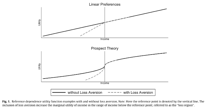
Aversion to falling below the reference point is consistent with loss aversion, with a result below the reference point causing stronger feelings than a result a similar amount above the reference point.
There have been numerous follow-up studies of taxi drivers. The results of these studies have varied.
Farber (2005) studied New York cab drivers and found that the decision to stop work was primarily a function of how many hours had been worked up to that point in the day. He identified the difference between his and Camerer et al.’s result as being due to different empirical methods and measurement problems with the Camerer et al. data.
Farber (2008) found that a labour supply model with reference-dependent targets better fits than a standard neoclassical model. However, there was substantial variation day-to-day in any given driver’s reference income level and most shifts ended before that reference income was reached.
Farber (2015) used a much larger dataset on New York taxi driver behaviour and found that, as standard economic theory would predict, taxi drivers drive more when they can earn more. Farber also found that drivers did not earn more when it was raining.
Finally, Martin (2017) examined taxi driver labour supply using the S-shaped reference dependence of prospect theory. That is, Martin used a model with the reflection effect, with risk-seeking behaviour in the loss domain and risk aversion in the gain domain. Martin found evidence that taxi driver behaviour was consistent with this full form of prospect theory. He differentiated from the other papers on the basis that they considered a narrower version of reference dependence focusing on loss aversion only.
19.3 The disposition effect
The disposition effect is the tendency for investors to sell stocks that are in the gain domain relative to the purchase price and to hold stocks that are in the loss domain.
While tax implications or portfolio rebalancing are both potential explanations for asymmetric behaviour relating to the sale of stocks, these factors are insufficient to explain the observed behaviour.
Most behavioural explanations have turned to prospect theory.
For example, Shefrin and Statman (1985) argued that the disposition effect is driven by the reflection effect, whereby investors are risk seeking in the loss domain and risk averse in the gain domain. To demonstrate how it works, they present the following scenario:
[C]onsider an investor who purchased a stock one month ago for $50 and who finds that the stock is now selling at $40. The investor must now decide whether to realize the loss or hold the stock for one more period. To simplify the discussion, assume that there are no taxes or transaction costs. In addition, suppose that one of two equiprobable outcomes will emerge during the coming period: either the stock will increase in price by $10 or decrease in price by $10. According to prospect theory, our investor frames his choice as a choice between the following two lotteries:
A. Sell the stock now, thereby realizing what had been a $10 “paper loss”.
B. Hold the stock for one more period, given 50-50 odds between losing an additional $10 or “breaking even.”
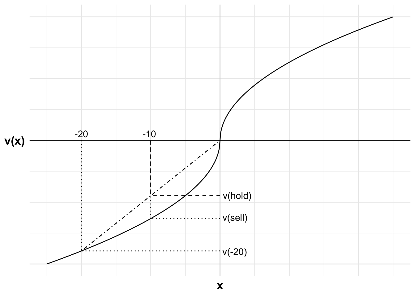
For an investor who is risk seeking in the loss domain, holding would be attractive. The following figure illustrates that the certain loss of $10 (from the reference point of $50) gives lower value than holding for a chance of eliminating the loss.
Code
library(ggplot2)u <-function(x){ifelse (x >=0, x^0.5, -(-x)^0.5)}df <-data.frame(x =seq(-25, 25, 0.1),y =u(seq(-25, 25, 0.1)))#Variables for plot (may not match labels as not done to scale)#Payoffs from gamblex1<--20#lossx2<-0#winev<--10#expected value of gamblexc<--10#certain outcomepx2<-(ev-x1)/(x2-x1)ggplot(mapping =aes(x, y)) +#Plot the utility curvegeom_line(data = df) +geom_vline(xintercept =0, linewidth=0.25)+geom_hline(yintercept =0, linewidth=0.25)+labs(x ="x", y ="v(x)")+# Set the themetheme_minimal()+#remove numbers on each axistheme(axis.text.x =element_blank(),axis.text.y =element_blank(),axis.title=element_text(size=14,face="bold"),axis.title.y =element_text(angle=0, vjust=0.5))+#limit to y greater than zero and x greater than -8 (need -8 so space for y-axis labels)coord_cartesian(xlim =c(-25, 25), ylim =c(-5, 5))+#Add labels -10, v(sell) and line to curve indicating eachannotate("text", x = xc, y =0, label ="-10", size =4, hjust =0.6, vjust =-0.5)+annotate("segment", x = xc, y =0, xend = xc, yend =u(xc), linewidth =0.5, colour ="black", linetype="dotted")+annotate("segment", x =0, y =u(xc), xend = xc, yend =u(xc), linewidth =0.5, colour ="black", linetype="dotted")+annotate("text", x =0, y =u(xc), label ="v(sell)", size =4, hjust =-0.1, vjust =0.3)+#Add labels -20, v(-20) and line to curve indicating eachannotate("text", x = x1, y =0, label ="-20", size =4, hjust =0.5, vjust =-0.5)+annotate("segment", x = x1, y =0, xend = x1, yend =u(x1), linewidth =0.5, colour ="black", linetype="dotted")+annotate("segment", x =0, y =u(x1), xend = x1, yend =u(x1), linewidth =0.5, colour ="black", linetype="dotted")+annotate("text", x =0, y =u(x1), label ="v(-20)", size =4, hjust =-0.1, vjust =0.6)+#Add expected utility lineannotate("segment", x = x1, xend = x2, y =u(x1), yend =u(x2), linewidth =0.5, colour ="black", linetype="dotdash")+#Add labels v(hold) and curve indicating positionannotate("segment", x = ev, y =0, xend = ev, yend =u(x1)+(u(x2)-u(x1))*px2, linewidth =0.5, colour ="black", linetype="dashed")+annotate("segment", x =0, y =u(x1)+(u(x2)-u(x1))*px2, xend = ev, yend =u(x1)+(u(x2)-u(x1))*px2, linewidth =0.5, colour ="black", linetype="dashed")+annotate("text", x =0, y =u(x1)+(u(x2)-u(x1))*px2, label ="v(hold)", size =4, hjust =-0.1, vjust =0.45)
Figure 19.1: The disposition effect in the loss domain
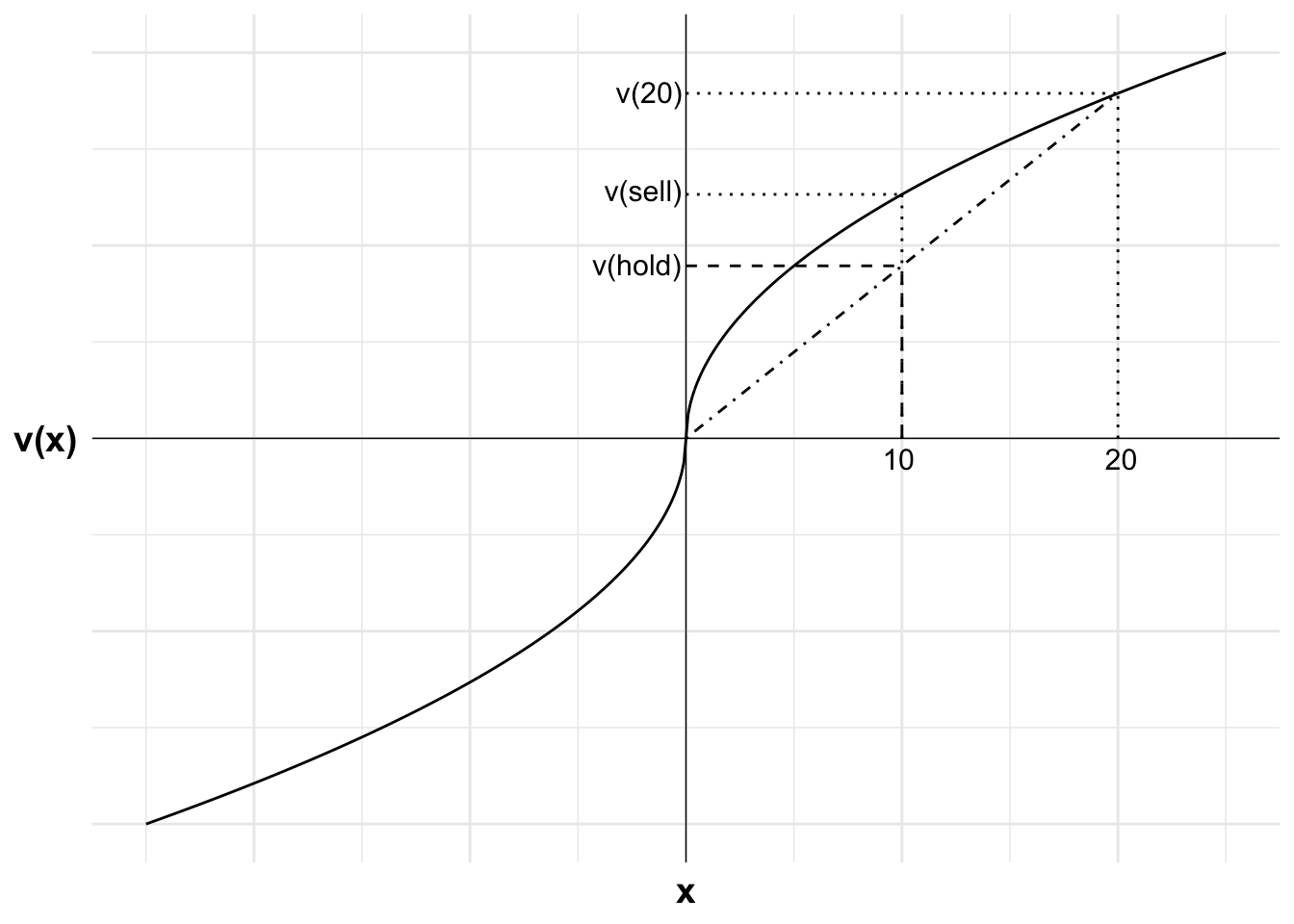
If we craft an alternative scenario where the stock is now selling at $60, selling would realise a $10 gain, while holding the stock would be a risky prospect with the same expected value. An investor who is risk averse in the gain domain will sell.
The following figure illustrates that the certain gain of $10 (from the reference point of $50) gives higher value than holding for a chance of a larger gain.
Code
library(ggplot2)u <-function(x){ifelse (x >=0, x^0.5, -(-x)^0.5)}df <-data.frame(x =seq(-25, 25, 0.1),y =u(seq(-25, 25, 0.1)))#Variables for plot (may not match labels as not done to scale)#Payoffs from gamblex1<-0#lossx2<-20#winev<-10#expected value of gamblexc<-10#certain outcomepx2<-(ev-x1)/(x2-x1)ggplot(mapping =aes(x, y)) +#Plot the utility curvegeom_line(data = df) +geom_vline(xintercept =0, linewidth=0.25)+geom_hline(yintercept =0, linewidth=0.25)+labs(x ="x", y ="v(x)")+# Set the themetheme_minimal()+#remove numbers on each axistheme(axis.text.x =element_blank(),axis.text.y =element_blank(),axis.title=element_text(size=14,face="bold"),axis.title.y =element_text(angle=0, vjust=0.5))+#limit to y greater than zero and x greater than -8 (need -8 so space for y-axis labels)coord_cartesian(xlim =c(-25, 25), ylim =c(-5, 5))+#Add labels 10, v(sell) and line to curve indicating eachannotate("text", x = xc, y =0, label ="10", size =4, hjust =0.6, vjust =1.5)+annotate("segment", x = xc, y =0, xend = xc, yend =u(xc), linewidth =0.5, colour ="black", linetype="dotted")+annotate("segment", x =0, y =u(xc), xend = xc, yend =u(xc), linewidth =0.5, colour ="black", linetype="dotted")+annotate("text", x =0, y =u(xc), label ="v(sell)", size =4, hjust =1.05, vjust =0.3)+#Add expected utility lineannotate("segment", x = x1, xend = x2, y =u(x1), yend =u(x2), linewidth =0.5, colour ="black", linetype="dotdash")+#Add labels 20, v(20) and line to curve indicating eachannotate("text", x = x2, y =0, label ="20", size =4, hjust =0.4, vjust =1.5)+annotate("segment", x = x2, y =0, xend = x2, yend =u(x2), linewidth =0.5, colour ="black", linetype="dotted")+annotate("segment", x =0, y =u(x2), xend = x2, yend =u(x2), linewidth =0.5, colour ="black", linetype="dotted")+annotate("text", x =0, y =u(x2), label ="v(20)", size =4, hjust =1.05, vjust =0.45)+#Add labels v(hold) and curve indicating positionannotate("segment", x = ev, y =0, xend = ev, yend =u(x1)+(u(x2)-u(x1))*px2, linewidth =0.5, colour ="black", linetype="dashed")+annotate("segment", x =0, y =u(x1)+(u(x2)-u(x1))*px2, xend = ev, yend =u(x1)+(u(x2)-u(x1))*px2, linewidth =0.5, colour ="black", linetype="dashed")+annotate("text", x =0, y =u(x1)+(u(x2)-u(x1))*px2, label ="v(hold)", size =4, hjust =1.05, vjust =0.45)
Figure 19.2: The disposition effect in the gain domain
19.4 The housing market
Genesove and Mayer (2001) examined housing data from Boston. They found that owners subject to nominal losses set higher asking prices, with the increase in asking price being 25% to 35% of the difference between the expected selling price and their original purchase price.
They also found that these owners attain higher prices, covering around 3% to 18% of that difference.
This suggests sellers are averse to realising nominal losses. However, note that the aversion leads to a better outcome.
Camerer, C., Babcock, L., Loewenstein, G., and Thaler, R. (1997). Labor supply of new york city cabdrivers: One day at a time*. The Quarterly Journal of Economics, 112(2), 407–441. https://doi.org/10.1162/003355397555244
Farber, H. S. (2005). Is tomorrow another day? The labor supply of new york city cabdrivers. Journal of Political Economy, 113(1), 46–82. https://doi.org/10.1086/426040
Farber, H. S. (2008). Reference-Dependent Preferences and Labor Supply: The Case of New York City Taxi Drivers. American Economic Review, 98(3), 1069–1082. https://doi.org/10.1257/aer.98.3.1069
Farber, H. S. (2015). Why you can’t find a taxi in the rain and other labor supply lessons from cab drivers. The Quarterly Journal of Economics, 130(4), 1975–2026. https://doi.org/10.1093/qje/qjv026
Genesove, D., and Mayer, C. (2001). Loss aversion and seller behavior: Evidence from the housing market. The Quarterly Journal of Economics, 116(4), 1233–1260. https://www.jstor.org/stable/2696458
Martin, V. (2017). When to quit: Narrow bracketing and reference dependence in taxi drivers. Journal of Economic Behavior & Organization, 144, 166–187. https://doi.org/10.1016/j.jebo.2017.09.024
Shefrin, H., and Statman, M. (1985). The Disposition to Sell Winners Too Early and Ride Losers Too Long: Theory and Evidence. The Journal of Finance, 40(3), 777–790. https://doi.org/10.1111/j.1540-6261.1985.tb05002.x