You are in a draw for $1 million. Consider the following four scenarios where your chances of winning increases by 5%:
From 0% to 5%
From 5% to 10%
From 50% to 55%
From 95% to 100%
Most people report that scenarios A) and D) represent better news. Why?
Answer
There is strong experimental evidence that we overweight certain events relative to near certain events. In this instance, we will tend to overweight the shift to a certain result (scenario D) relative to shifts involving intermediate probabilities (e.g. scenario B and C). This overweighting of certainty is effectively the same as overweighting low probability events. As a result, the probability shift that provides an initial chance at $1 million is also overweighted (scenario A).
The result is that scenarios A and D tend to be seen as better news than scenarios B and C.
The following diagram illustrates. On the horizontal axis is the probability (p). On the vertical axis is the decision weight applied to each probability (\pi). If people applied probability weights linearly as they do in expected utility theory, the dashed line would represent how probabilities map to weights. Under prospect theory, people overweight small probabilities and underweight probabilities short of certainty. The solid line represents one functional mapping of these possibility and certainty effects.
From this diagram, you can then see the change in decision weight from each change in probability. The changes from 0% to 5% and from 95% to 100% represent much larger changes in decision weight than the changes in intermediate probabilities.
20.2 Bitcoin
Edna, Ferdinand and Gretel each bought some Bitcoin at $50,000. The price rose to $80,000 and then dropped to $60,000, at which time they sold it.
All three are loss averse and have the following reference-dependent value function:
v(x)=\left\{\begin{matrix}
x \quad &\textrm{where} \quad x \geq 0\\
2x \quad &\textrm{where} \quad x < 0
\end{matrix}\right.
Edna uses the purchase price as her reference point. Ferdinand uses the peak price as his reference point. Gretel uses the sale price as her reference point.
What is the change in value for each person? Who is happiest?
Edna is happiest whereas Ferdinand is most disappointed. Both Edna and Gretel see the peak price as a foregone gain, whereas Ferdinand sees the failure to sell at the peak as a loss.
20.3 Reference points
Megan has the following reference-dependent value function:
v(x)=\left\{\begin{matrix}
x \quad &\textrm{where} \quad x \geq 0\\
2x \quad &\textrm{where} \quad x < 0
\end{matrix}\right.
where x is the realised outcome relative to the reference point.
a) If you look at v(x), we expect Megan to be:
loss averse
have no decreased sensitivity to changes of greater magnitude.
Why?
Answer
Megan is loss averse as the slope of the value function in the loss domain is steeper than in the gain domain. One unit of loss leads to a greater change in value than one unit of gain.
There is no decreases sensitivity as the value function is linear in both domains. Sensitivity is constant. As the size of the loss or gain increases, the change in value remains constant despite the increasing magnitude.
b) Assume Megan has received a birthday card from her aunt, which some years contains $25 and other years contains nothing.
She opens the card and it contains $10.
Consider two alternative reference points: Megan is pessimistic and expects no money in the card, and Megan is optimistic and expects $25.
Compute Megan’s value under each reference point. Which reference point yields higher value?
Answer
The value of the $10 from the reference point of expecting nothing is:
Megan has higher value when she does not expect to receive any money. She gets the value of a gain of $10. If she expected the $25, she suffered the value of a loss of $15.
c) Megan has received the $10 in the card and a piece of birthday cake. Her value function over money and pieces of birthday cake is:
v(x)=v(m-r_m)+v(4c-4r_c)
Where m is the amount of money she receives, r_m is her reference point of how much money she expects, c is how many pieces of birthday cake she receives and r_c is how many pieces of birthday cake she expects.
To illustrate how this value function works, imagine Megan expects two pieces of cake and her dog jumps onto the table and eats one of them. Her change in the value function is:
For this question, assume Megan does not believe that she will receive any money and she expects to eat two pieces of birthday cake. Her reference point is therefore r_m=0 and r_c=2. She receives $10 from her aunt.
Her brother - who loves cake - offers to buy one of her pieces of birthday cake. What price p_s would make Megan indifferent between selling and keeping the piece of cake?
Answer
Megan will be indifferent when the value from each option is the same:
d) Assume that Megan expects to receive only one piece of birthday cake. Her brother then offers to sell her his piece of cake. For r_m=0 and r_c=1, what price p_b would make Megan indifferent between buying the cake and eating only her own piece?
Answer
Megan will be indifferent when the value from each option is the same:
e) Why is there a difference between the price at which Megan was willing to sell cake in part c) compared to the price she was willing to pay in part d)?
Answer
The willingness to accept in part c) is higher than the willingness to pay in part d) as in part c) the foregone cake is coded as a loss. This loss reduces value at twice the rate of a gain in cake. The payment for the cake in both parts is in the gain domain due to the birthday present of $10, so the payment received or paid is given less weight than any loss.
20.4 Saving on a purchase
Consider the following two scenarios:
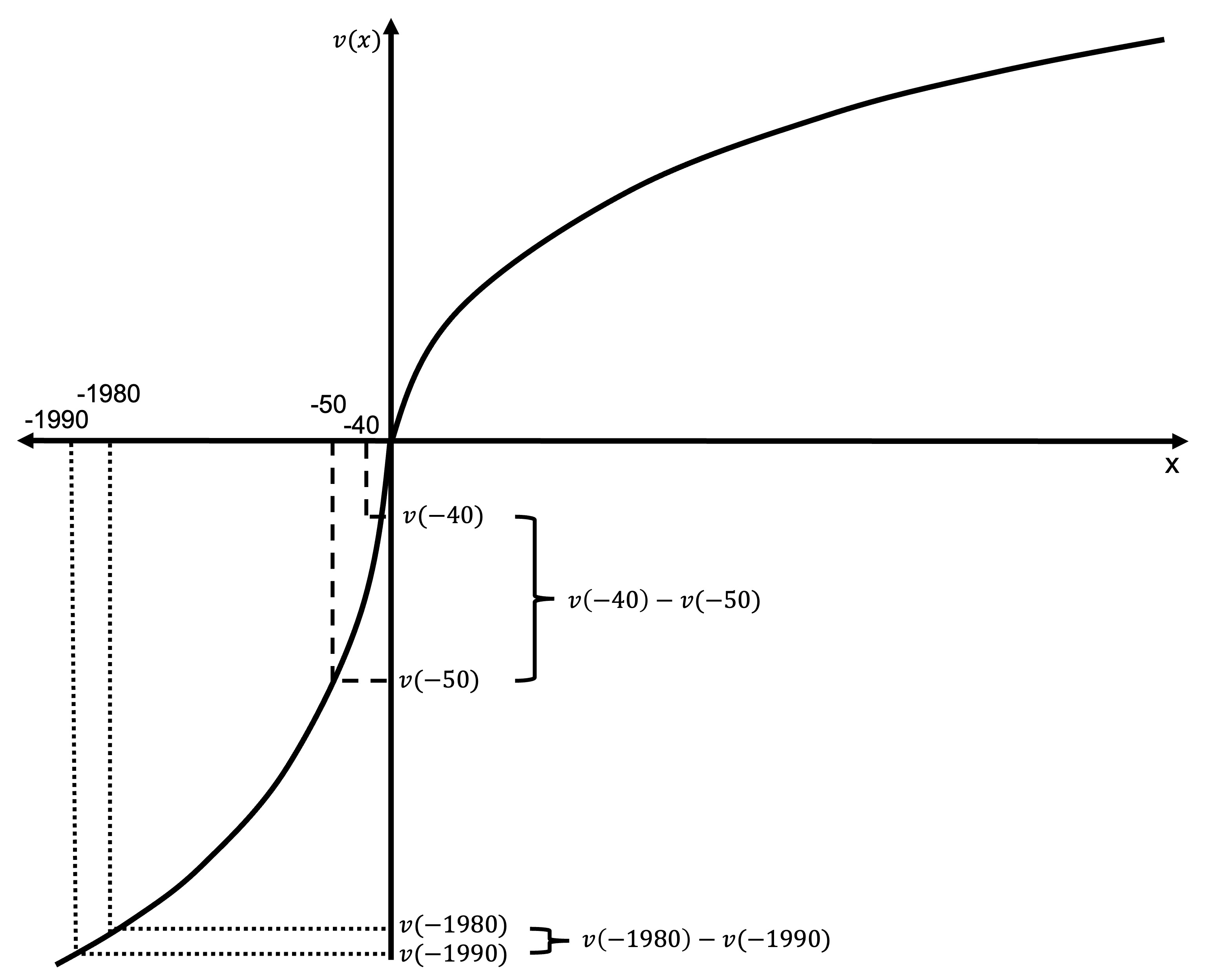
A) You are considering buying a new type of coffee bean for your home coffee machine. It costs $50 at your local hipster cafe, but you discover that it is for sale for $40 at the supermarket 20 minutes drive from your home. Do you make the trip?
B) You are considering buying a new laptop. It costs $1990 at your local computer store, but you discover that it is for sale for $1980 at another computer store 20 minutes drive from your home. Do you make the trip?
When people are presented with scenarios such as this, they tend to report that they are less likely to make the trip in Scenario B for the more expensive product.
Explain how an S-shaped value function with diminishing value in both gains and losses could result in this behaviour.
Answer
Diminishing value means that the absolute difference between v(-40) and v(-50) is much larger than the absolute difference between v(-1980) and v(-1990). For example, suppose the value function was:
v(x)=\left\{\begin{matrix}
x^\frac{1}{2} \quad &\textrm{where} \quad x \geq 0\\
-2(-x)^\frac{1}{2} \quad &\textrm{where} \quad x < 0
\end{matrix}\right.
This would mean that the difference between v(-40) and v(-50) is:
They will not want to play this gamble as it has a negative value for the agent. They could receive value of 0 by simply not playing.
The reason for this negative value is that the agent is loss averse. The loss of $100 is given twice the weight of an equivalent gain, meaning that they reject the bet despite a win of $100 being more probable.
b) Suppose the agent takes this gamble and loses $100. They feel bad about it and perceive it as a loss. Their reference point is unchanged at the original status quo. They are offered gamble A again? Do they accept this second time? Why?
Answer
After losing $100 but not changing their reference point, they have two possible outcomes relative to their reference point: recovery of their loss of $100 so they come out even and a loss of $200 (losing $100 twice).
They will now want to play the gamble as it has a greater value than staying with their current loss. The reason the gamble becomes attractive is because it gives an opportunity to recover the loss. The agent is risk seeking over the loss domain.
c) The agent is offered a new job for which they receive a $50,000 sign-on bonus. They adapt to their new wealth, so their reference point changes to accommodate their new situation. They are now offered gamble A again. Do they accept? Why?
Answer
With their new reference point, this question is effectively the same as part a). They will refuse the bet.
20.6 A 50:50 gamble
Suppose Tim has the following reference-dependent value function:
v(x)=\left\{\begin{matrix}
x^{1/2} \qquad &\textrm{where} &\space x \geq 0\\
-2(-x)^{1/2} \quad &\textrm{where} &\space x < 0
\end{matrix}\right.
x is the change in Tim’s position relative to his reference point.
a) What feature of Tim’s value function leads to loss aversion? Explain.
Answer
The part of the value function that applies when x<0 is increased by a factor of two relative to that part of the value function for when x>0. This is done by multiplying the bottom portion by 2.
b) Tim considers the gamble A: ($250, 0.5; -$100, 0.5). Will Tim want to play this gamble?
Tim has negative value from the gamble, when he could simply have zero value by declining. He rejects.
c) Explain what features of the value function lead him to accept or reject the gamble.
Answer
Two features of the value function lead him to reject:
Tim is loss averse (the -2 in the bottom equation), which leads him to give twice the weight to losses relative to an equal sized gain.
Tim has diminishing sensitivity to losses and gains. The larger gain is reduced proportionately more by this diminishing sensitivity.
d) Suppose Tim were to experience a large positive or negative shock to his wealth that does not immediately change his reference point. Could either shock cause him to change his decision concerning gamble A? Explain.
Answer
Both a positive and negative shock could lead Tim to change his decision.
A large positive shock would place the entire bet into the gain domain. That would remove loss aversion as a factor in rejecting the bet. Given the high expected value, that would likely be sufficient for him to accept. However, a large shock would also place Tim further up the value function to a region where it is more linear (i.e. he is less risk averse). This will also increase the tendency to accept the bet.
A large negative shock would place the entire bet into the loss domain. That would remove loss aversion as a factor in rejecting the bet as there is no gain against which the loss can be given relatively greater weight. Due to diminishing sensitivity to losses, Tim is also risk seeking in the loss domain. This would lead him to accept any bet with a positive expected value.
20.7 Insurance AND gambling
Explain how probability weighting as proposed under Prospect Theory can lead a person to simultaneously gamble and purchase insurance.
Answer
Decisions under Prospect Theory are the outcome of two factors:
The value function that gives a value to each outcome relative to a reference point
The probability weighting function that gives a decision weight to the probability of each outcome.
The Prospect Theory value function leads people to be risk averse in the domain of gains and risk seeking in the loss domain. This combination would tend to lead people to purchase neither insurance or lotteries. Their risk seeking behaviour could lead them to avoid the certain loss of the insurance premium. They would rather risk the loss of the insurable asset.
Code
library(ggplot2)u <-function(x){ifelse (x >=0, x^0.5, -2*(-x)^0.5)}df <-data.frame(x =seq(-220, 220, 0.1),y =u(seq(-220, 220, 0.1)))#Variables for plot (may not match labels as not done to scale)#Payoffs from gamblex1<--200#lossx2<-0#winev<--30#expected value of gamblexc<--60#certain outcomepx2<-(ev-x1)/(x2-x1)ggplot(mapping =aes(x, y)) +#Plot the utility curvegeom_line(data = df) +geom_vline(xintercept =0, linewidth=0.25)+geom_hline(yintercept =0, linewidth=0.25)+labs(x ="x", y ="v(x)")+# Set the themetheme_minimal()+#remove numbers on each axistheme(axis.text.x =element_blank(),axis.text.y =element_blank(),axis.title=element_text(size=14,face="bold"),axis.title.y =element_text(angle=0, vjust=0.5))+#limit to y greater than zero and x greater than -8 (need -8 so space for y-axis labels)coord_cartesian(xlim =c(-220, 220), ylim =c(-30, 15))+#Add labels -V, v(L) and line to curve indicating eachannotate("text", x = x1, y =0, label ="-V", size =4, hjust =0.5, vjust =-0.3)+annotate("segment", x = x1, y =0, xend = x1, yend =u(x1), linewidth =0.5, colour ="black", linetype="dotted")+annotate("segment", x =0, y =u(x1), xend = x1, yend =u(x1), linewidth =0.5, colour ="black", linetype="dotted")+annotate("text", x =0, y =u(x1), label ="v(-V)", size =4, hjust =-0.1, vjust =0.6)+#Add labels -P, v(-P) and line to curve indicating eachannotate("text", x = xc, y =0, label ="-P", size =4, hjust =0.8, vjust =-0.3)+annotate("segment", x = xc, y =0, xend = xc, yend =u(xc), linewidth =0.5, colour ="black", linetype="dotted")+annotate("segment", x =0, y =u(xc), xend = xc, yend =u(xc), linewidth =0.5, colour ="black", linetype="dotted")+annotate("text", x =0, y =u(xc), label ="v(-P)", size =4, hjust =-0.1, vjust =0.3)+#Add expected utility lineannotate("segment", x = x1, xend = x2, y =u(x1), yend =u(x2), linewidth =0.5, colour ="black", linetype="dotdash")+#Add labels E[don't], v(don't) and curve indicating eachannotate("text", x = ev, y =0, label ="E[don't]", size =4, hjust =0.5, vjust =-0.3)+annotate("segment", x = ev, y =0, xend = ev, yend =u(x1)+(u(x2)-u(x1))*px2, linewidth =0.5, colour ="black", linetype="dashed")+annotate("segment", x =0, y =u(x1)+(u(x2)-u(x1))*px2, xend = ev, yend =u(x1)+(u(x2)-u(x1))*px2, linewidth =0.5, colour ="black", linetype="dashed")+annotate("text", x =0, y =u(x1)+(u(x2)-u(x1))*px2, label ="v(don't)", size =4, hjust =-0.1, vjust =0.45)
Figure 20.1: Purchasing insurance
Their risk averse behaviour in the domain of gains would make a lottery with a negative expected value unattractive, as the following diagram shows (not drawn to scale - the relative size of a win would typically dwarf the ticket price).
Code
u <-function(x){ifelse (x >=0, x^0.5, -2*(-x)^0.5)}df <-data.frame(x =seq(-110, 160, 0.1),y =u(seq(-110, 160, 0.1)))#Variables for plot (may not match labels as not done to scale)#Payoffs from gamblex1 <--50#lossx2 <-150#winev <-0.2*x2+0.8*x1 #expected value of gamblexc <-0#certain outcomepx2<-(ev-x1)/(x2-x1)ggplot(mapping =aes(x, y)) +#Plot the utility curvegeom_line(data = df) +geom_vline(xintercept =0, linewidth=0.25)+geom_hline(yintercept =0, linewidth=0.25)+labs(x ="x", y ="v(x)")+# Set the themetheme_minimal()+#remove numbers on each axistheme(axis.text.x =element_blank(),axis.text.y =element_blank(),axis.title=element_text(size=14,face="bold"),axis.title.y =element_text(angle=0, vjust=0.5))+#limit to y greater than zero and x greater than -8 (need -8 so space for y-axis labels)coord_cartesian(xlim =c(-80, 160), ylim =c(-15, 15))+#Add labels -T, v(-T) and line to curve indicating eachannotate("text", x = x1, y =0, label ="-T", size =4, hjust =0.5, vjust =-0.5)+annotate("segment", x = x1, y =0, xend = x1, yend =u(x1), linewidth =0.5, colour ="black", linetype="dotted")+annotate("segment", x =0, y =u(x1), xend = x1, yend =u(x1), linewidth =0.5, colour ="black", linetype="dotted")+annotate("text", x =0, y =u(x1), label ="v(-T)", size =4, hjust =-0.1, vjust =0.45)+#Add expected utility lineannotate("segment", x = x1, xend = x2, y =u(x1), yend =u(x2), linewidth =0.5, colour ="black", linetype="dotdash")+#Add labels W-T, v(W-T) and line to curve indicating eachannotate("text", x = x2, y =0, label ="W-T", size =4, hjust =0.4, vjust =1.5)+annotate("segment", x = x2, y =0, xend = x2, yend =u(x2), linewidth =0.5, colour ="black", linetype="dotted")+annotate("segment", x =0, y =u(x2), xend = x2, yend =u(x2), linewidth =0.5, colour ="black", linetype="dotted")+annotate("text", x =0, y =u(x2), label ="v(W-T)", size =4, hjust =1.05, vjust =0.45)+#Add labels E[A], V(A) and curve indicating eachannotate("text", x = ev, y =0, label ="E[X]", size =4, hjust =0.4, vjust =-0.5)+annotate("segment", x = ev, y =0, xend = ev, yend =u(x1)+(u(x2)-u(x1))*px2, linewidth =0.5, colour ="black", linetype="dashed")+annotate("segment", x =0, y =u(x1)+(u(x2)-u(x1))*px2, xend = ev, yend =u(x1)+(u(x2)-u(x1))*px2, linewidth =0.5, colour ="black", linetype="dashed")+annotate("text", x =0, y =u(x1)+(u(x2)-u(x1))*px2, label ="V(X)", size =4, hjust =-0.1, vjust =0.45)
Figure 20.2: Purchasing a lottery
However, the probability weighting function can counteract that effect. By overweighting the small probability of an insurable event or a lottery win, the agent may decide to insure or purchase a lottery despite the risk attitudes inherent in the value function.
As an example, consider an agent who overweights a probability of 1 in a million lottery win by 1,000 times, acting as though they would win the $1 million prize once every 1000 lotteries. They also overweight the probability of a one in a thousand fire that would destroy their million dollar house by 100 times, acting as though it is a 1-in-10 chance. (These numbers are extreme, but I am creating a toy example.)
Suppose the lottery ticket is $1 and their utility function is:
They purchase insurance as it has higher value than not purchasing it.
20.8 Locking in a win
Amber sued a tabloid newspaper for defamation. The trial has completed and the judge has retired to make her decision.
Amber’s lawyer tells her that she has a 95% chance of winning and receiving $1,000,000 in damages, meaning she has a 5% chance of leaving with nothing. (Ignore any potential costs.) She then receives an offer of settlement from the newspaper for $800,000. Amber accepts.
Use the fourfold pattern of attitudes to risk under prospect theory to explore why Amber accepted the settlement offer.
Answer
Rejecting the offer has a higher expected value than the value of the settlement:
Two forces under prospect theory would lead Amber to take the option with the lower expected value:
People are risk averse in the gain domain. Amber would prefer certainty to a gamble with the same expected value, and depending on the level of risk aversion, would be willing to accept an amount for certain lower than the expected value of the bet. That is, the certainty equivalent of the gamble would be less than its expected value.
People overweight small probabilities. The 5% probability of losing is likely overweighted by Amber.
20.9 Lotteries as incentives
A common intervention to encourage behaviour change is to offer a lottery ticket as an incentive. For example, a lottery ticket might be offered to people who complete a survey.
The government is considering whether it should incentivise vaccination with either:
a payment of $10 or
a lottery ticket with a 1 in a million chance of winning $10 million.
Use concepts from prospect theory to explain why either option might be more successful.
Answer
There are two opposing forces that could lead to either option being preferred.
Both the lottery and payment of $10 are in the gain domain. Under prospect theory, people tend to be risk averse in the gain domain. This will make the payment, which has the same expected value as the lottery, more attractive.
Conversely, under prospect theory, people do not weight outcomes directly by their probability. They apply decision weights that tend to overweight small probabilities and underweight probabilities just short of certainty. This means that the small chance of $10 million will likely be overweighted. This could lead to the value of the lottery exceeding that of a certain payment.
Which effect dominates depends on how risk-averse people are and how much they overweight the probability.