As V(A) > V(-\$100), Lisa will prefer the gamble to the certain $100 loss.
Another way to think about this problem is to calculate the certainty equivalent of gamble A and compare that to the certain loss. The certainty equivalent is the amount of money that Lisa would be indifferent between receiving for certain and the gamble. A benefit of calculating the certainty equivalent is that you can then easily determine whether Lisa would prefer the gamble to a certain loss of any particular amount.
The certainty equivalent (CE) of gamble A is calculated as:
The certainty equivalent of gamble A is a loss of $90. Lisa would be indifferent between losing $90 for certain and the gamble. For any loss greater than $90, Lisa would prefer the gamble. Given this information, we can say that Lisa will prefer the gamble to the certain loss of $100.
(c) Explain what features of the value function leads Lisa to accept or reject the gamble.
Answer
The bet has a lower expected value (a loss of $150) relative to the certain outcome of a loss of $100. Lisa would need to be risk seeking to find the bet attractive.
Lisa’s diminishing sensitivity to losses leads her to be risk seeking in the loss domain, which is where the gamble is located. This is why she prefers the gamble to a certain loss.
Loss aversion does not affect her decision, as all possible outcomes (at least under our assumed reference point) are in the loss domain.
(d) Draw a diagram illustrating the choice in part (b). Show the possible payoffs, Lisa’s value function and the value of each option. Explain how this diagram illustrates Lisa’s decision.
Answer
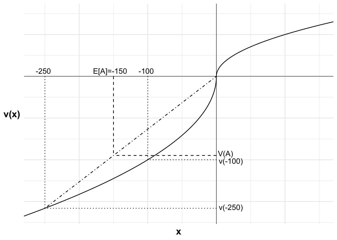
The diagram below shows the possible payoffs, Lisa’s value function and the value of each option.
The possible outcomes from the gamble are zero and a loss of $250. The certain outcome on offer is a loss of $100. The expected value of the gamble is 0.6\times -\$250+0.4\times 0=-\$150.
As Lisa is risk seeking, the value of the certain $100 loss is lower than the weighted value of the gamble. This can be seen through v(A) being greater than v(-\$100). Lisa will, therefore, choose the gamble.
Code
library(ggplot2)u <-function(x){ifelse (x >=0, x^0.5, -2*(-x)^0.5)}df <-data.frame(x =seq(-300, 300, 0.1),y =u(seq(-300, 300, 0.1)))#Variables for plot (may not match labels as not necessarily done to scale)#Payoffs from gamblex1<--250#lossx2<-0#winev<--150#expected value of gamblexc<--100#certain outcomepx2<-(ev-x1)/(x2-x1)ggplot(mapping =aes(x, y)) +#Plot the utility curvegeom_line(data = df) +geom_vline(xintercept =0, linewidth=0.25)+geom_hline(yintercept =0, linewidth=0.25)+labs(x ="x", y ="v(x)")+# Set the themetheme_minimal()+#remove numbers on each axistheme(axis.text.x =element_blank(),axis.text.y =element_blank(),axis.title=element_text(size=14,face="bold"),axis.title.y =element_text(angle=0, vjust=0.5))+#limit to y greater than zero and x greater than -8 (need -8 so space for y-axis labels)coord_cartesian(xlim =c(-260, 150), ylim =c(-33, 15))+#Add labels -250, v(-250) and line to curve indicating eachannotate("text", x = x1, y =0, label ="-250", size =4, hjust =0.6, vjust =-0.5)+annotate("segment", x = x1, y =0, xend = x1, yend =u(x1), linewidth =0.5, colour ="black", linetype="dotted")+annotate("segment", x =0, y =u(x1), xend = x1, yend =u(x1), linewidth =0.5, colour ="black", linetype="dotted")+annotate("text", x =0, y =u(x1), label ="v(-250)", size =4, hjust =-0.1, vjust =0.3)+#Add labels -100, v(-100) and line to curve indicating eachannotate("text", x = xc, y =0, label ="-100", size =4, hjust =0.6, vjust =-0.5)+annotate("segment", x = xc, y =0, xend = xc, yend =u(xc), linewidth =0.5, colour ="black", linetype="dotted")+annotate("segment", x =0, y =u(xc), xend = xc, yend =u(xc), linewidth =0.5, colour ="black", linetype="dotted")+annotate("text", x =0, y =u(xc), label ="v(-100)", size =4, hjust =-0.1, vjust =0.7)+#Add expected utility lineannotate("segment", x = x1, xend = x2, y =u(x1), yend =u(x2), linewidth =0.5, colour ="black", linetype="dotdash")+#Add labels 0, v(0) and line to curve indicating each#annotate("text", x = x2, y = 0, label = "0", size = 4, hjust = 0.4, vjust = 1.5)+#annotate("segment", x = x2, y = 0, xend = x2, yend = u(x2), linewidth = 0.5, colour = "black", linetype="dotted")+#annotate("segment", x = 0, y = u(x2), xend = x2, yend = u(x2), linewidth = 0.5, colour = "black", linetype="dotted")+#annotate("text", x = 0, y = u(x2), label = "v(0)", size = 4, hjust = 1.05, vjust = 0.45)+#Add labels E[A], V(A) and curve indicating eachannotate("text", x = ev, y =0, label ="E[A]=-150", size =4, hjust =0.6, vjust =-0.5)+annotate("segment", x = ev, y =0, xend = ev, yend =u(x1)+(u(x2)-u(x1))*px2, linewidth =0.5, colour ="black", linetype="dashed")+annotate("segment", x =0, y =u(x1)+(u(x2)-u(x1))*px2, xend = ev, yend =u(x1)+(u(x2)-u(x1))*px2, linewidth =0.5, colour ="black", linetype="dashed")+annotate("text", x =0, y =u(x1)+(u(x2)-u(x1))*px2, label ="V(A)", size =4, hjust =-0.1, vjust =0.1)
Figure 54.1
(e) Suppose Lisa were to win $100 in a raffle. The win does not change her reference point. Could this win cause her to change her decision concerning the loss of $100 and gamble A?
As V(A) < V(-\$100), Lisa will prefer the certain loss.
(f) Explain what features of the value function lead Lisa to accept or reject the gamble in part (e). How does this differ from your answer in part (c)?
Answer
The bet has a lower expected value (a loss of $150) relative to the certain outcome of a loss of $100. Or to put it another way, the expected outcome of the gamble relative to her reference point (a loss of $50) is less than the certain outcome of $0 relative to her reference point.
Therefore, Lisa would need to be risk seeking across most of the relevant domain to find the bet attractive. She is risk seeking across some of the domain (loss), but risk averse across some (gain). The net result of that curvature is an insufficient level of risk seeking to make the bet attractive.
Similarly, loss aversion makes the bet less attractive, but it would still be rejected even in the absence of loss aversion. (We can see this by calculating the weighted value of the gamble without the loss aversion multiplier.)
(g) Draw a diagram illustrating the choices in parts (e). Show the possible payoffs, Lisa’s value function and the value of each option. Explain how this diagram illustrates Lisa’s decision after the raffle win.
Answer
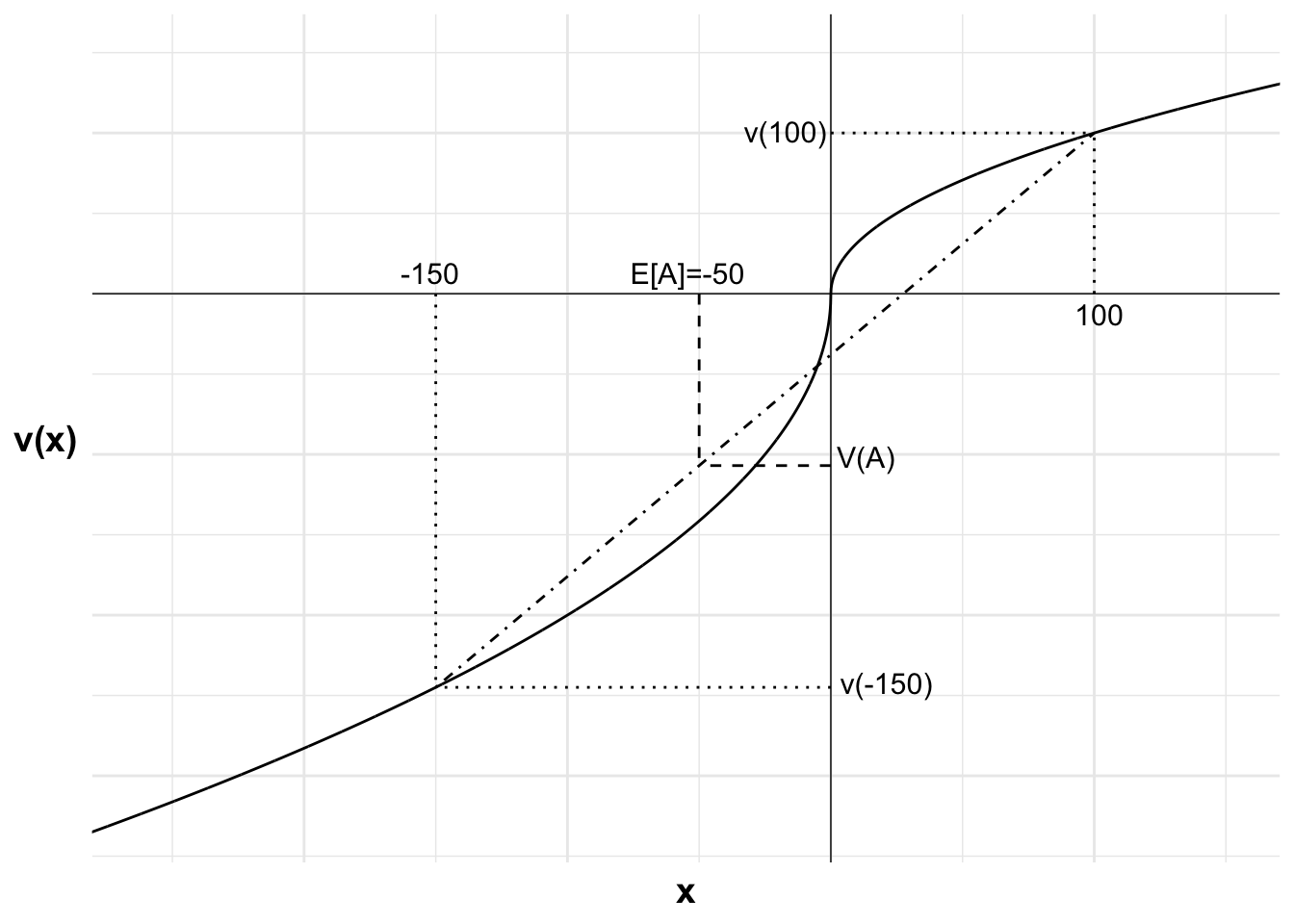
This diagram illustrates Lisa’s decision after the win.
The possible outcomes from the gamble relative to the reference point are a gain of $100 (a loss of zero plus the $100 win) and a loss of $150 (a loss of $250 plus the $100 win). The certain outcome on offer is zero (a certain loss of $100 plus the $100 win). The expected value of the outcome after the gamble is 0.6\times -\$150+0.4\times 100=-\$50.
As the bet has negative expecrted value, plus Lisa is loss averse, V(A) is less than the alternative outcome of zero.
Code
library(ggplot2)u <-function(x){ifelse (x >=0, x^0.5, -2*(-x)^0.5)}df <-data.frame(x =seq(-300, 300, 0.1),y =u(seq(-300, 300, 0.1)))#Variables for plot (may not match labels as not necessarily done to scale)#Payoffs from gamblex1<--150#lossx2<-100#winev<--50#expected value of gamblexc<-0#certain outcomepx2<-(ev-x1)/(x2-x1)ggplot(mapping =aes(x, y)) +#Plot the utility curvegeom_line(data = df) +geom_vline(xintercept =0, linewidth=0.25)+geom_hline(yintercept =0, linewidth=0.25)+labs(x ="x", y ="v(x)")+# Set the themetheme_minimal()+#remove numbers on each axistheme(axis.text.x =element_blank(),axis.text.y =element_blank(),axis.title=element_text(size=14,face="bold"),axis.title.y =element_text(angle=0, vjust=0.5))+#limit to y greater than zero and x greater than -8 (need -8 so space for y-axis labels)coord_cartesian(xlim =c(-260, 150), ylim =c(-33, 15))+#Add labels -150, v(-150) and line to curve indicating eachannotate("text", x = x1, y =0, label ="-150", size =4, hjust =0.6, vjust =-0.5)+annotate("segment", x = x1, y =0, xend = x1, yend =u(x1), linewidth =0.5, colour ="black", linetype="dotted")+annotate("segment", x =0, y =u(x1), xend = x1, yend =u(x1), linewidth =0.5, colour ="black", linetype="dotted")+annotate("text", x =0, y =u(x1), label ="v(-150)", size =4, hjust =-0.1, vjust =0.3)+#Add labels -100, v(-100) and line to curve indicating each#annotate("text", x = xc, y = 0, label = "-100", size = 4, hjust = 0.6, vjust = -0.5)+#annotate("segment", x = xc, y = 0, xend = xc, yend = u(xc), linewidth = 0.5, colour = "black", linetype="dotted")+#annotate("segment", x = 0, y = u(xc), xend = xc, yend = u(xc), linewidth = 0.5, colour = "black", linetype="dotted")+#annotate("text", x = 0, y = u(xc), label = "v(-100)", size = 4, hjust = -0.1, vjust = 0.7)+#Add expected utility lineannotate("segment", x = x1, xend = x2, y =u(x1), yend =u(x2), linewidth =0.5, colour ="black", linetype="dotdash")+#Add labels 100, v(1000) and line to curve indicating eachannotate("text", x = x2, y =0, label ="100", size =4, hjust =0.4, vjust =1.5)+annotate("segment", x = x2, y =0, xend = x2, yend =u(x2), linewidth =0.5, colour ="black", linetype="dotted")+annotate("segment", x =0, y =u(x2), xend = x2, yend =u(x2), linewidth =0.5, colour ="black", linetype="dotted")+annotate("text", x =0, y =u(x2), label ="v(100)", size =4, hjust =1.05, vjust =0.45)+#Add labels E[A], V(A) and curve indicating eachannotate("text", x = ev, y =0, label ="E[A]=-50", size =4, hjust =0.6, vjust =-0.5)+annotate("segment", x = ev, y =0, xend = ev, yend =u(x1)+(u(x2)-u(x1))*px2, linewidth =0.5, colour ="black", linetype="dashed")+annotate("segment", x =0, y =u(x1)+(u(x2)-u(x1))*px2, xend = ev, yend =u(x1)+(u(x2)-u(x1))*px2, linewidth =0.5, colour ="black", linetype="dashed")+annotate("text", x =0, y =u(x1)+(u(x2)-u(x1))*px2, label ="V(A)", size =4, hjust =-0.1, vjust =0.1)
Figure 54.2: Lisa’s consideration of gamble A and the $100 loss after the win
54.2 Question 2
Early in the COVID-19 pandemic, the hope was that vaccines would prevent transmission and death. Later, it became apparent that vaccination dramatically reduced death rates but did not wholly prevent it.
Use the concept of probability weighting to explain why citizens would see a massive reduction as much less valuable than elimination.
Answer
There is strong evidence that we overweight certain events, when the probability of the event is one, relative to near certain events, such as when the probability is, say, 99%. This overweighting of certainty is effectively the same as overweighting very low-probability events.
The elimination of COVID-19 would be seen as a certain event, and therefore overweighted relative to a near-certain event, such as a 99% reduction in deaths. Hence elimination would be seen as much more valuable even though near-elimination has nearly the same number of lives saved
Put another way, the remaining small probability of death would be overweighted, meaning the near elimination of deaths would be seen as having much less value than the complete elimination.