The following examples demonstrate how understanding intertemporal choice can inform policy design and product development to help individuals overcome present bias and achieve long-term goals.
People willingly choose illiquid savings accounts with equal or lower interest rates, suggesting demand for commitment devices among sophisticated, present-biased agents.
A voluntary commitment product involving forfeitable deposits increased the likelihood of quitting smoking, demonstrating the effectiveness of commitment devices in behaviour change.
Default effects significantly influence organ donor registration rates, potentially due to present bias or rational cost-benefit calculations.
The Save More Tomorrow program successfully increases retirement savings by mitigating loss aversion and present bias.
ANZ Bank’s Progress Saver and Term Deposit accounts illustrate how present bias and the demand for commitment devices influence consumer financial decisions.
29.1 Introduction
In this part, I discuss several applications of the intertemporal choice concepts we have covered.
29.2 Savings
The first example relates to the use of commitment devices to increase savings.
Beshears et al. (2020) offered experimental participants the opportunity to save in two accounts, one liquid and the other with liquidity constraints such as withdrawal penalties. They found that the experimental participants put nearly half of their money in the illiquid account even though it paid the same interest rate. This behaviour contrasts with the standard economic prediction that all money should go to the liquid account, which dominates the illiquid account’s features. Even when the interest rate on the illiquid account was lower, it still attracted around a quarter of the money.
This extract from Table 3 in the paper shows the proportion of funds allocated to each type of “commitment account” when experimental participants had a choice between an account with no liquidity constraints paying 22% interest and the commitment account.
You can see that where the interest rates between the liquid and illiquid accounts were equal, the accounts with harsher constraints attracted more money. The account with a higher withdrawal penalty (20% compared to 10%) attracted more money, and the account that barred withdrawals attracted even more.
This result suggests a demand among sophisticated, present-biased agents for products that will enable them to control their future behaviours.
This behaviour has also been observed outside the lab.
Ashraf et al. (2006) offered a commitment savings product called SEED (Save, Earn, Enjoy Deposits) to randomly chosen clients of a Philippine bank. SEED restricted access to savings for one year.
Other than providing a possible commitment savings device, no further benefit accrued to individuals with this account.
Despite this, 28% of participants took up a commitment savings product. The average savings balance increased by 42% after six months and 82% after one year.
29.3 Smoking
The following example relates to quitting smoking.
Giné et al. (2010) tested a voluntary commitment product for smoking cessation.
Smokers were offered a product that comprised a savings account in which they deposit funds. After six months, they took urine tests for nicotine and cotinine.
If they passed, the money was returned. Otherwise, it was forfeited.
The result was that 11% of smokers offered the product took it up. Smokers offered the product were 3 percentage points more likely to pass the 6-month test than the control group
The effect persisted in a surprise test at 12 months.
29.4 Organ donation
The next example concerns organ donation.
In European countries there are registers of people who will donate their organs in case of death. There is a considerable gap in the percentage of registered organ donors between countries. Why?
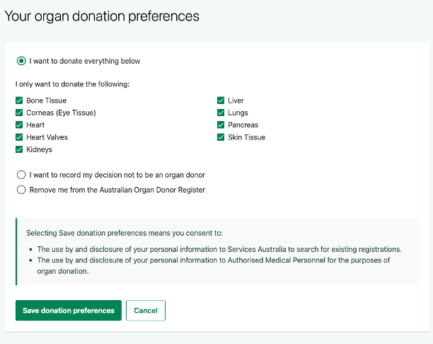
Yellow countries have an opt-in policy. People are required to register as an organ donor.
Green countries have an opt-out policy known as presumed consent. Citizens are presumed to consent unless they opt out (often through submission of a form).
This outcome is a classic example of a default effect. Defaults are sticky. The stickiness of defaults is typically assumed to come from loss aversion or present bias.
Present bias might influence the decision as follows. There is an immediate cost of changing from the default, be that time, effort or money. That cost is not discounted. In contrast, the future benefit of their action is discounted.
If you asked these people about their future plans, they might say they intend to change their organ donation registration. In the hypothetical, both the costs and benefits and in the future. They believe they will switch later.
However, it is possible to argue that the stickiness of the defaults is due to a rational cost-benefit calculation rather than loss aversion or present bias. The cost of opting out is real, and people may not have a strong preference about whether they are an organ donor.
Further, registration does not mean that your organs will be donated. Other factors, such as family preference, affect donation. Among other things, the absence of any active consent in situations of presumed consent means that the family cannot take the organ donation register as an indication of the deceased’s wishes. There is little benefit in changing the registration if it will have little effect on the outcome you care about (actual organ donation).
Johnson and Goldstein (2003) argued that there is a positive relationship between an opt-out policy and organ donations. But, it is much weaker than the registration numbers would suggest and based on a simple regression that likely does not capture all relevant variables.
There are alternatives to presumed consent that may increase organ donation rates.
One alternative is using defaults more transparently with easy opt out. For example, when obtaining your driver’s licence, there could be a section stating: “Please tick this box if you do not wish to be registered as an organ donor”. This measure would likely increase registration over the alternative of asking people to tick the box if they wish to be an organ donor.
Another alternative is “active choice”, where citizens are required to indicate whether or not they wish to be registered. This choice could also be built into a form such as a driver’s licence application or renewal.
29.5 Save More Tomorrow
The next example of intertemporal choice relates to retirement savings.
The Save More Tomorrow program, designed by Thaler and Benartzi (2004), combines prospect theory and time preference principles to increase retirement savings.
Under Save More Tomorrow, customers are asked to commit in advance to allocating a fraction of their future salary increases toward their retirement savings accounts.
Save More Tomorrow is designed to reduce loss aversion when deciding contribution amounts. A commitment of a proportion of a pay rise means that the contribution can increase over time, but pay never decreases.
The program is designed to reduce the effect of present bias. The cost of the savings is in the future, meaning that the costs are subject to the short-term discount factor and not disproportionately overweighted relative to the benefits.
The program capitalises on participants’ propensity to stick with the status quo, as people are unlikely to unwind their future commitments despite being able to opt out at any time.
That ability to opt out also reduces regret and disappointment aversion.
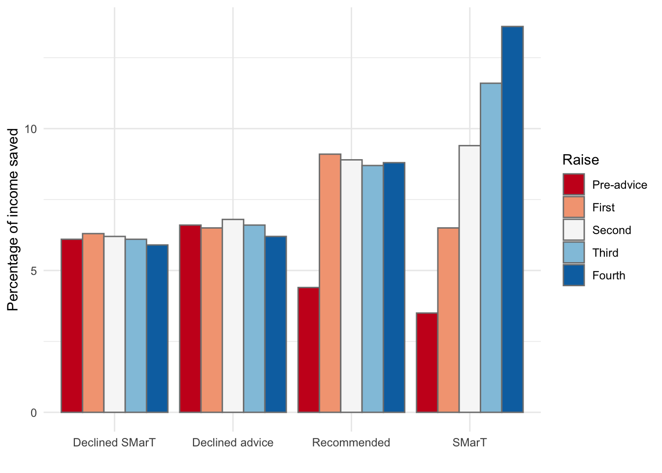
The first tests of the Save More Tomorrow program by Thaler and Benartzi (2004) resulted in 78 per cent of those offered the plan joining, 80 per cent of those remaining in the plan through the fourth pay rise, and average savings rates increasing from 3.5 per cent to 13.6 per cent over 40 months. This compares to much lower savings rates by those who declined advice, accepted a recommended savings rate or took advice but declined to enrol in Save More Tomorrow.
Figure 29.1 illustrates the results. Along the horizontal axis are the four groups: those who declined to enrol in the program, those who declined to receive advice, those who accepted a recommended savings rate, and those who accepted the Save More Tomorrow program. The vertical axis shows the percentage of income saved at each of five measurement points; before they received advice and after the following four raises.
Code
library(ggplot2)library(dplyr)library(tidyr)df <-data.frame( "Raise"=c("Pre-advice", "First", "Second", "Third", "Fourth"),"Declined-advice"=c(6.6, 6.5, 6.8, 6.6, 6.2),"Recommended"=c(4.4, 9.1, 8.9, 8.7, 8.8),"SMarT"=c(3.5, 6.5, 9.4, 11.6, 13.6),"Declined"=c(6.1, 6.3, 6.2, 6.1, 5.9) )df2 <- df |>pivot_longer(!Raise, names_to ="group", values_to ="percentage") |>arrange(group) |>mutate(Raise=factor(Raise, levels=c("Pre-advice", "First", "Second", "Third", "Fourth")))df2 <- df2[,c(2,1,3)]df2 <- df2 |>mutate(group =replace(group, group =="No.advice", "Declined advice")) |>mutate(group =replace(group, group =="Declined", "Declined SMarT"))ggplot(df2, aes(group, percentage)) +geom_col(aes(group = Raise, fill=Raise), colour ="grey50", position ="dodge")+labs(x ="", y ="Percentage of income saved") +scale_fill_brewer(palette="RdBu")+#change Declined.advice to Declined advicescale_x_discrete(labels =function(x) gsub("Declined.advice", "Declined advice", x))+# Set the themetheme_minimal()
Figure 29.1: Savings rates for SMarT
Note the savings rate is higher than the default rate in Australia. Could the default in Australia create a low anchor for some people?
29.6 The Progress Saver Account
Another applied example of how we can use intertemporal choice in an applied setting concerns ANZ bank’s progress saver account.
ANZ bank’s progress saver account pays bonus monthly interest on the condition that a customer deposits at least $10 into the account and makes no withdrawals. The bonus interest was 3.74% per year at the time of writing. If you fail to make the minimum deposit or withdraw from the account, you are paid a nominal interest rate of 0.01% per year on your savings for the month.
Many account holders do not receive bonus interest each month. Most notably, while they often make deposits, they later withdraw funds, leading to the loss of the bonus interest.
This behaviour may be evidence of a preference reversal due to present bias. Today, the customer may have a preference for saving money for a long-term goal rather than short-term spending at a closer date. But when that opportunity for spending arrives, they prefer withdrawing from the account and spending the money now. That spending is no longer subject to the short-term discount factor \beta, whereas the long-term savings goal and any interest toward achieving it are.
For example, suppose a customer is deciding whether to save money for their house deposit far in the future or spend the money on a new pair of shoes when they go shopping next week. Both are in the future and are subject to a short-term discount factor. In that circumstance, saving for the deposit might be preferred. However, when the shopping day comes, the shoes can be bought now. The shoes are not subject to the short-term discount factor and may give higher discounted utility than the long-term savings goal. The customer then withdraws the funds for the shoes, having changed their mind.
The behaviour could also be for rational reasons, such as a change in circumstances.
The bank has another product, a term deposit savings account, that pays, at the time of writing, 0.15% interest if you commit your money for 12 months. Many customers still use the term deposit despite paying much lower interest than the progress saver account and constraining access to funds.
Why do people use this apparently sub-optimal product?
Some customers are what we call “sophisticated” present-biased agents. They are present biased, but they know they are present biased. They can see their future failings as they think through problems using backward induction. As a result, they can implement strategies to restrain their future self, such as a commitment device. A commitment device is a mechanism that locks you into a course of action by changing the value or availability of future options.
If they foresaw spending their money on shoes, they would know that depositing in the progress saver account would not lead to them saving for their house deposit long term. As a result, that person may decide to forgo the possibility of higher interest (that they won’t receive) to constrain their future self from buying shoes when shopping. The term deposit provides that constraint, acting as a commitment device.
Ashraf, N., Karlan, D., and Yin, W. (2006). Tying odysseus to the mast: Evidence from a commitment savings product in the philippines*. The Quarterly Journal of Economics, 121(2), 635–672. https://doi.org/10.1162/qjec.2006.121.2.635
Beshears, J., Choi, J. J., Harris, C., Laibson, D., Madrian, B. C., and Sakong, J. (2020). Which early withdrawal penalty attracts the most deposits to a commitment savings account? Journal of Public Economics, 183, 104144. https://doi.org/10.1016/j.jpubeco.2020.104144
Giné, X., Karlan, D., and Zinman, J. (2010). Put Your Money Where Your Butt Is: A Commitment Contract for Smoking Cessation. American Economic Journal: Applied Economics, 2(4), 213–235. https://doi.org/10.1257/app.2.4.213
Thaler, Richard H., and Benartzi, S. (2004). Save More Tomorrow: Using Behavioral Economics to Increase Employee Saving. Journal of Political Economy, 112(S1), S164–S187. https://doi.org/10.1086/380085
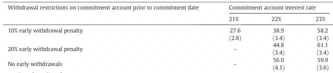
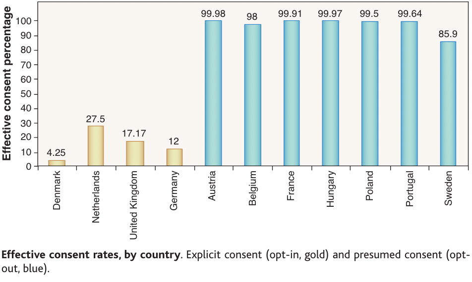 Figure from