The following examples illustrate the contrast between exponential discounters’ time-consistent choices and present-biased agents’ time-inconsistent decisions when faced with immediate versus future rewards.
The use of graphical representations to visualise how present bias affects the relative attractiveness of rewards over time, particularly when the short-term discount factor no longer applies, can be used to illustrate choice and preference reversal.
The following examples illustrate that:
The \beta\delta model creates a “kink” in the discounting curve, with a steeper discount for the immediate future due to the short-term discount factor \beta.
Present-biased agents may choose smaller-sooner rewards when available immediately, but larger-later rewards when both options are in the future.
Present bias has practical implications in financial decision-making, demonstrated through scenarios such as loan repayment choices.
25.2 Introduction
In the section, I provide some simple examples of the \beta\delta model.
25.3 Exponential discounting versus present bias
For the first example, we will consider the following pair of choices presented to an exponential discounting agent and a present-biased agent and contrast their decisions.
Choice 1: Would you like $100 today or $110 next week?
Choice 2: Would you like $100 next week or $110 in two weeks?
25.3.1 The exponential discounter
The exponential discounter has \delta=0.95 and utility each period of u(x_n)=x_n.
Would the exponential discounter prefer $100 today (t=0) or $110 next week (t=1)?
When we worked through this problem in Section 22.2, we calculated that:
U_0(0,\$100)=100<104.5=U_0(1,\$110)
The exponential discounter will prefer to receive $110 next week as it leads to higher discounted utility.
Choice 2: Would the exponential discounter prefer $100 next week (t=1) or $110 in two weeks (t=2)?
When we worked through this problem in Section 22.2, we calculated that:
U_0(1,\$100)=95<99.275=U_0(2,\$110)
The exponential discounter will prefer to receive $110 in two weeks.
The set of decisions across Choice 1 and Choice 2 are time consistent. If the exponential-discounting agent selected $110 in two weeks for Choice 2 and was given a chance to change their choice after one week (which is effectively an offer of Choice 1), they would not change their decision.
25.3.2 The present-biased agent
The present biased agent has \delta=0.95, \beta=0.95 and utility each period of u(x_n)=x_n.
Choice 1: Would this agent prefer $100 today (t=0) or $110 next week (t=1)?
As U_0(1,\$100)=90.25<94.31=U_0(2,\$110), the present-biased agent will prefer to receive $110 in two weeks.
If we consider those two choices by the present-biased agent together, we see the following pattern.
For choice 1, the present-biased agent will prefer $100 now to $110 in one week. Their preference for benefits now due to the short-term discount factor \beta leads them to prefer the immediate payoff.
For choice 2, the present-biased agent will prefer $110 in two weeks to $100 in one week. They are willing to wait longer for a larger reward, with both outcomes in the future and subject to the short-term discount factor \beta.
Consider what would happen if this present-biased agent selected the $110 in two weeks in Choice 2, but after one week we asked if they would like to reconsider their choice. They are effectively being offered Choice 1. This would then lead them to change their mind and take the immediate $100.
This combination of decisions is time inconsistent. The present-biased agent’s actions are not consistent with their initial plan.
We can see this change in preference in the following diagram.
The vertical bars represent the payments of $100 and $110. The lines projecting back from the bars to the y-axis represent the discounted utility of each payment at each time.
There is a kink in the line projecting from the $110 in two weeks, representing the effect of the short-term discount factor \beta. Between t=1 and t=2 both the short-term and usual discount factors are applied. This leads to that part of the curve having a steeper slope than between t=0 and t=1 where only the usual discount factor is applied.
At t=0 the discounted utility of the $110 at t=2 is higher and that payment is therefore preferred. At t=1 when the $100 is no longer discounted by the short-term discount factor \beta, it suddenly becomes more attractive. If offered on that day, would be chosen in substitute of the $110 due in another week.
Code
# Create a function to create the discounted bar chartlibrary(ggplot2)# Helper function to create discounted valuescreate_discount_data <-function(value, t, beta, delta, start) { times <-seq(start, t, by =1)data.frame(t = times,group =as.character(t),value =ifelse(t==times, value, value * beta * delta^(t - times)) )}# Main function to create the discounted bar chartcreate_discounted_bar_chart <-function(smaller, t_s, larger, t_l, beta, delta, starting_at =0, y_spacing =20, x_spacing =1) {# Create the data data <-data.frame(t =c(t_s, t_l),U_t =c(smaller, larger) )# Create the discounted values, starting from 'starting_at' discounted_data <-rbind(create_discount_data(smaller, t_s, beta, delta, starting_at),create_discount_data(larger, t_l, beta, delta, starting_at) )# Shift t values based on starting_at data$t_plot <- data$t - starting_at discounted_data$t_plot <- discounted_data$t - starting_at# Filter out any data points before the starting point data <- data[data$t >= starting_at, ] discounted_data <- discounted_data[discounted_data$t >= starting_at, ]# Determine x-axis and y-axis limits x_min <-0 x_max <-max(max(data$t_plot), max(discounted_data$t_plot)) y_max <-max(max(data$U_t), max(discounted_data$value)) *1.1# 10% buffer# Create the plotggplot() +# Add the barsgeom_rect(data = data, aes(xmin =ifelse(t_plot ==0, 0, t_plot -0.15),xmax =ifelse(t_plot ==0, 0.15, t_plot +0.15),ymin =0, ymax = U_t),fill ="white", color ="black") +# Add the discount linesgeom_line(data = discounted_data, aes(x = t_plot, y = value, group = group, linetype = group), color ="black", linewidth =1) +# Customize the plotscale_x_continuous(breaks =seq(x_min, x_max +1, by = x_spacing), limits =c(x_min, x_max +1),expand =c(0, 0),labels =function(x) x + starting_at) +scale_y_continuous(breaks =seq(0, y_max, by = y_spacing), limits =c(0, y_max),expand =c(0, 0)) +geom_vline(xintercept =0, linewidth =0.25) +geom_hline(yintercept =0, linewidth =0.25) +labs(x ="t",y =expression(U[t])) +theme_minimal() +theme(axis.title.y =element_text(angle =0, vjust =0.5),panel.grid.major =element_blank(),panel.grid.minor =element_blank(),legend.position ="none" )}
As U_5(5,\$10)=10>8.86=U_5(10,\$20), this present-biased agent will prefer to receive $10 today. They have changed their preference between the two payments relative to their decision at t=0.
We can see this change in preference in the following diagram.
The vertical bars represent the payments of $10 and $20. The lines projecting back from the bars to the y-axis represent the discounted utility of each payment at each time. There is a kink in the line in the period immediately before each payment, representing the effect of the short-term discount factor \beta.
At t=0 (and through to t=4) the discounted utility of the $20 at t=10 is higher and that payment is therefore preferred. At t=5 when the $10 is no longer discounted by the short-term discount factor \beta, it suddenly becomes more attractive. If offered on that day, would be chosen in substitute of the $20 due in another five days.
Charlie is a naive present-biased agent with \beta=0.5, \delta=0.95 and u(x)=x.
Charlie loaned $100 to Carol. Carol is due to pay Charlie back in 7 days (at t=7). Carol tells Charlie that she would prefer to pay him back later, and offers $200 in 14 days (at t=14) if he is willing to wait. Charlie is considering whether to accept Carol’s offer.
(a) What does Charlie choose at t=0?
To determine what Charlie chooses at t=0, we need to compare the discounted utility of the two options.
Charlie chooses the option with the highest discounted utility, which is $200 at t=14.
(b) At t=7 Charlie considers whether he should now demand payment of $100 at t=7 rather than wait for payment of $200 at t=14. What does Charlie choose at t=7?
To determine what Charlie chooses at t=7, we need to compare the discounted utility of the two options.
Charlie chooses the option with the highest discounted utility, which is $100 at t=7. He has changed his mind. This is because the sum at t=7 is no longer subject to the short-term discount factor \beta.
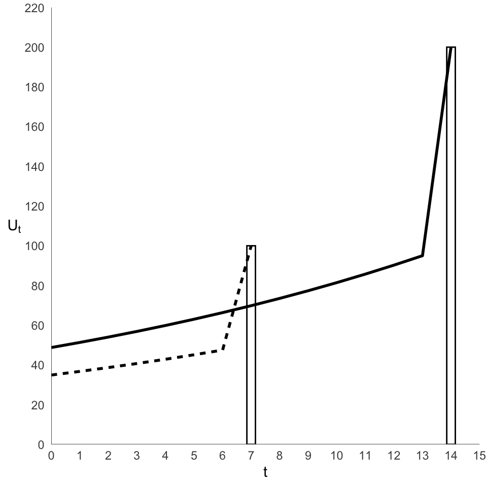
(c) Draw a graph illustrating Charlie’s choices.
The following chart shows each of the two options presented to Charlie, $100 at t=7 and $200 at t=14. The line extended from each back to t=0 represents the the discounted utility of each option at time t.
It can be seen that from t=0 to t=6, the discounted utility of $200 at t=14 is higher than the discounted utility of $100 at t=7. However, at t=7, the discounted utility of $100 at t=7 is higher than the discounted utility of $200 at t=14. Hence Charlie changes his mind.