Prospect theory’s value function incorporates three phenomena: reference dependence, loss aversion, and the reflection effect.
The function is defined on changes relative to a reference point, rather than final wealth levels, with diminishing marginal sensitivity to both gains and losses.
The value function is characterised by a kink at the reference point, with losses weighted more heavily than gains.
15.1 Introduction
The three phenomena, reference dependence, loss aversion and the reflection effect, are each incorporated into the prospect theory value function.
First, the value function of prospect theory is defined on changes in wealth or welfare rather than on final wealth levels. In other words, gains and losses are defined relative to a reference point. The reference point might be the status quo, lagged consumption, a goal, or an expectation about the outcome.
Utility from an outcome depends on the distance to the relevant reference level. A multi-millionaire may reject a 50:50 bet to win $550, lose $500 because they are not comparing the outcomes to their total wealth but rather are making a judgment relative to the reference point of the status quo.
Second, perceptions of both gains and losses are characterised by diminishing marginal sensitivity in either direction. Successive incremental changes have a smaller marginal impact.
This is similar to decreasing marginal utility of wealth in expected utility theory. Prospect theory and expected utility theory differ in the baseline. In expected utility theory, the starting value is typically zero wealth, with increases from there decreasing in marginal utility. In prospect theory, the starting value is the reference point, with both increases and decreases having smaller marginal effects as they increase in magnitude.
Third, losses loom larger than gains. People feel more strongly about a loss than they do an equivalent gain. They are often willing to reject gambles with a materially positive expected value.
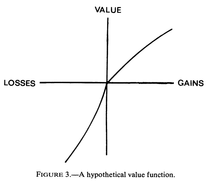
These phenomena result in the following famous figure from Kahneman and Tversky (1979).
1. The value function is centred on the reference point at the origin
2. There is a kink at the origin, with losses counting more than gains.
3. There is diminishing sensitivity to further changes from the reference point in both directions.
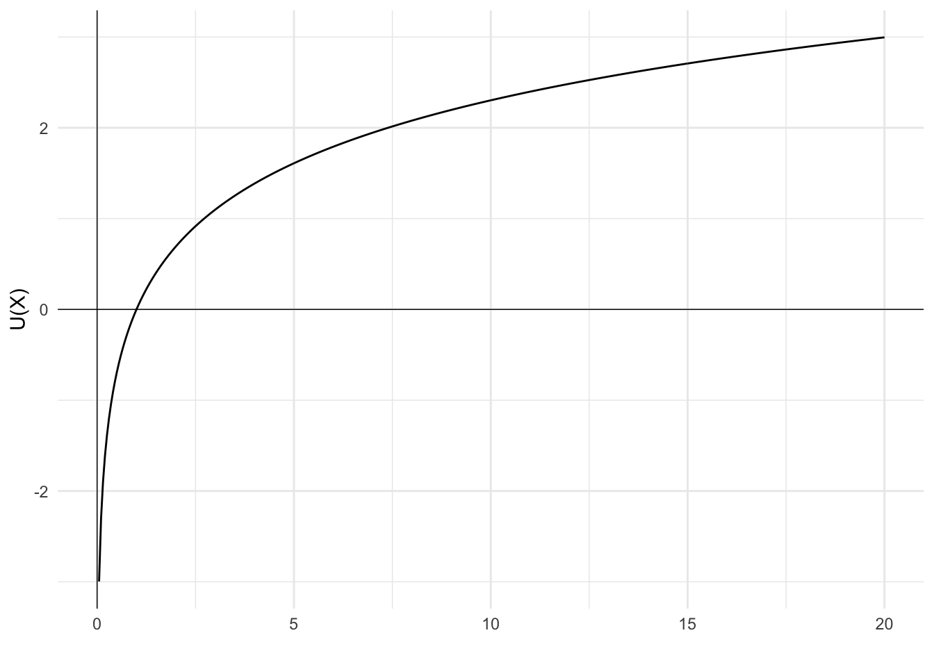
The following diagrams illustrate the different shapes of the expected utility function and the Prospect Theory value function.
The expected utility function, in this case U(x)=ln(x), has diminishing marginal utility as utility increases. Utility is measured from a reference point of zero.
Code
library(ggplot2)df <-data.frame(x =seq(0.05,20,0.05),y=NA)df$y <-log(df$x)ggplot(mapping =aes(x, y))+geom_line(data = df)+geom_vline(xintercept =0, linewidth=0.25)+geom_hline(yintercept =0, linewidth=0.25)+labs(x ="", y ="U(X)")+# Set the themetheme_minimal()
Figure 15.1: Expected utility function
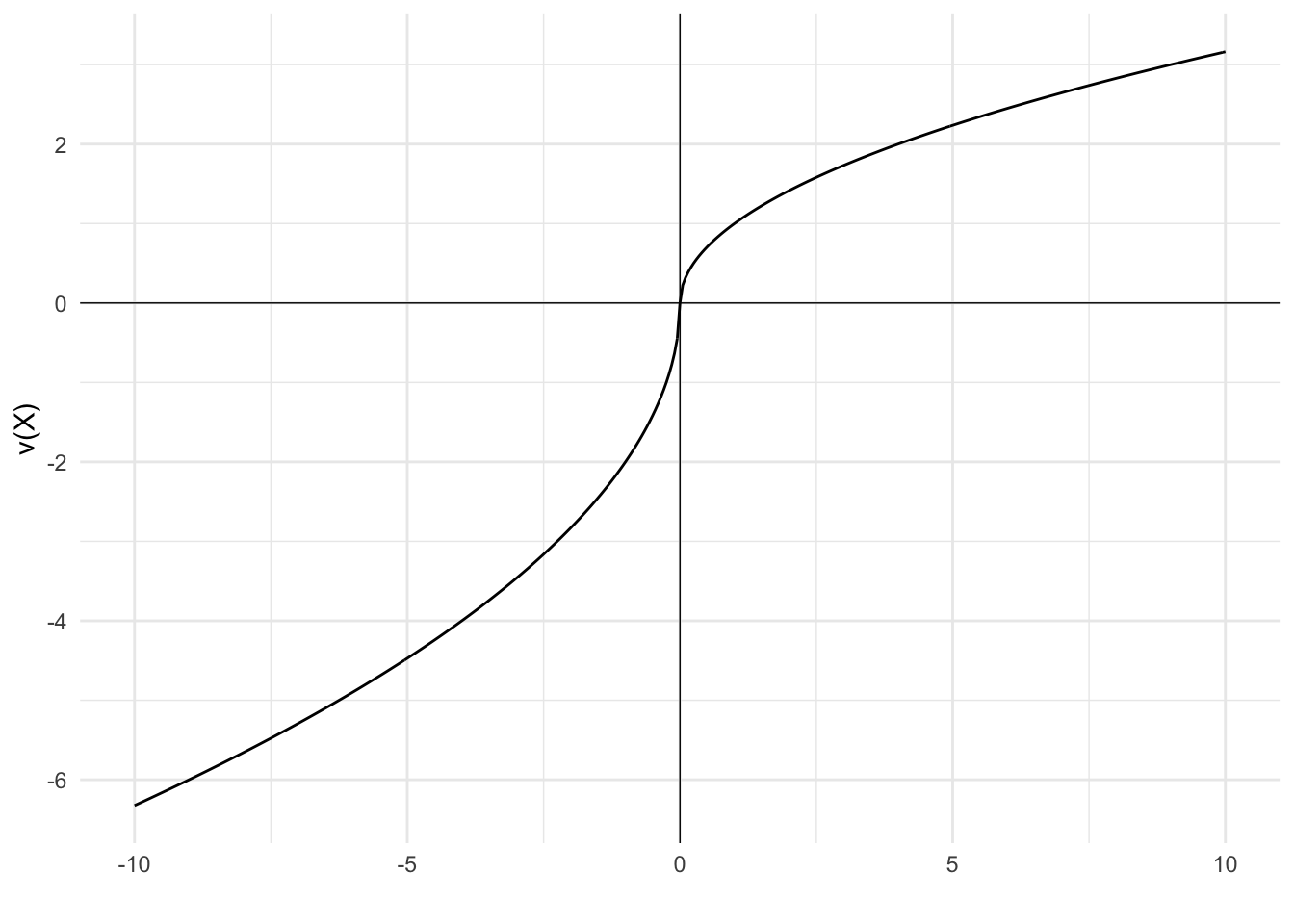
For the prospect theory function, you can see the kink at zero, with losses weighted more heavily than gains, with gains and losses determined relative to a reference point. There is diminishing sensitivity to further changes in both directions
Code
loss_fun <-function(x){#| -2*(-x)^0.5}gain_fun <-function(x){ x^0.5}loss <-data.frame(x=seq(-10,0,0.05),y=NA )loss$y <-loss_fun(loss$x)gain <-data.frame(x=seq(0,10,0.05),y=NA )gain$y <-gain_fun(gain$x)ggplot(mapping =aes(x, y)) +geom_line(data = loss) +geom_line(data = gain) +geom_vline(xintercept =0, linewidth=0.25)+geom_hline(yintercept =0, linewidth=0.25)+labs(x ="", y ="v(X)")+# Set the themetheme_minimal()
Figure 15.2: Prospect theory value function
The following equation is an example of a value function incorporating both loss aversion and the reflection effect.
Losses are multiplied by 2, giving losses twice the weight of an equivalent gain in the value function. This is loss aversion.
The reflection effect is implemented through losses and gains being to the power of one-half. This leads to diminishing sensitivity to changes in both directions.
Kahneman, D., and Tversky, A. (1979). Prospect theory: An analysis of decision under risk. Econometrica, 47(2), 263–291. https://doi.org/10.2307/1914185