The Allais Paradox demonstrates that people’s choices between pairs of bets often violate expected utility theory, as their preferences can be inconsistent when a common consequence (a shared outcome with equal probability in both options) is changed.
Rejection of small-scale bets implies unreasonably high risk aversion for larger bets under expected utility theory. For example, rejecting a 50:50 bet to win $110 or lose $100 at all wealth levels implies rejecting a 50:50 bet to win $1 billion or lose $1,000.
People’s choices are influenced by how options are framed, contradicting expected utility theory’s assumption of description invariance.
People evaluate outcomes relative to reference points rather than absolute wealth.
In this part, I show several anomalies in expected utility theory.
11.1 The Allais Paradox
The Allais paradox is one of the most famous anomalies in expected utility theory.
The paradox was first identified by Maurice Allais (1953). It emerges from the pattern of response to two pairs of bets. The following example comes from Kahneman and Tversky (1979).
For choice 1, the player is asked to choose one of the following bets:
Under Bet A, the player wins:
$2500 with probability 33%
$2400 with probability 66%
$0 with probability 1%
Under Bet B, the player wins:
$2400 with probability 100%
Which do you prefer?
When Kahneman and Tversky (1979) ran this experiment, 82% of participants chose option B.
For choice 2, the player is again asked to choose one of two bets:
Under Bet C, the player wins:
$2500 with probability 33%
$0 with probability 67%
Under Bet D, the player wins:
$2400 with probability 34%
$0 with probability 66%
Which do you prefer?
When Kahneman and Tversky (1979) ran this experiment, 83% of participants chose option C.
Let’s examine this pair of preferences, with over 80% of experimental participants selecting B in Choice 1 and C in Choice 2.
According to expected utility theory, if an agent selects B, the expected utility of B must be greater than the expected utility of A. That is:
U(2400)>0.33U(2500)+0.66U(2400)+0.01U(0)
We can simplify that to:
0.34U(2400)>0.33U(2500)+0.01U(0)
We can do the same analysis with the second choice. According to expected utility theory, if an agent selects C, the expected utility of C must be greater than the expected utility of D. That is:
0.33U(2500)+0.67U(0)> 0.34U(2400)+ 0.66U(0)
We can simplify that to:
0.33U(2500)+0.01U(0)> 0.34U(2400)
This is a contradiction. The two inequalities point in opposite directions. Under expected utility theory, if an agent chooses A it should choose C. And if the agent chooses B, it should choose D.
Why does this occur? What axiom is being breached?
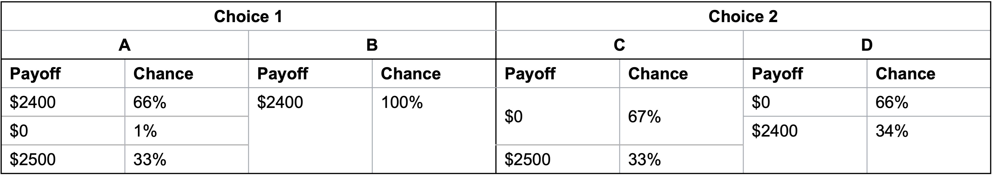
To understand this, I will show you another representation of the choices in this table. The left half of the table shows the bets for choice 1, and the right half for choice 2. Within each choice, the bets are represented as a payoff-chance pair. For example, I can read from the table that bet A involves a 66% chance of $2400, a 1% chance of $0, and a 33% chance of $2500. Bet B involves a 100% chance of $2400.
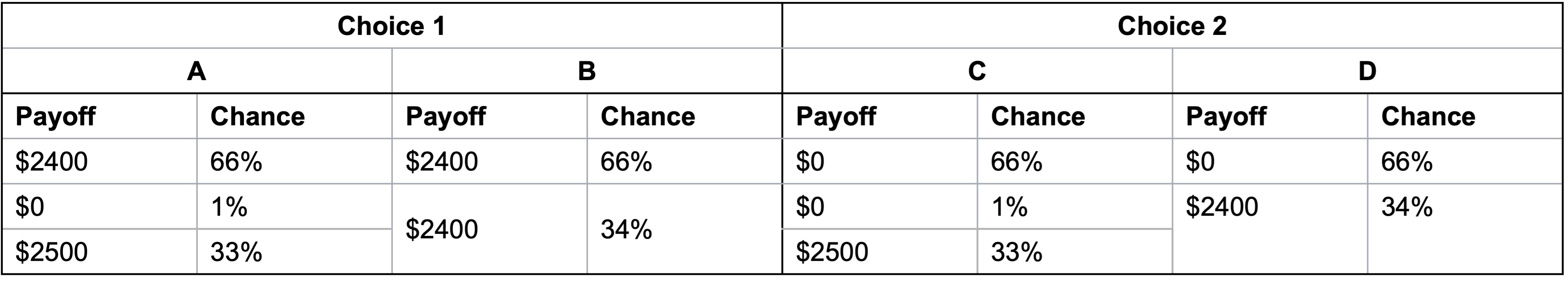
I can then break up these payoff-chance pairs to create an equivalent representation as in this second table. I have split the outcomes in bets B and C. For example, I have written the 100% chance of $2400 in option B as a 66% chance of $2400 and a 34% chance of $2400. I have written the 67% chance of $0 in bet C as a 66% chance of $0 and a 1% chance of $0.
With this split, you can see that the bets in the bottom two rows of choice 1 and choice 2 are the same. Both choice 1 and choice 2 involve a choice between, in one bet, a 1% chance of nothing and a 33% chance of $2,500 and in the other bet, a 34% chance of $2,400.
That shared bet in choice 1 and choice 2 is paired with a 66% chance of the same payoff regardless of the preferred bet. For choice 1 that “common consequence” across bet A and bet B is $2400. For choice 2, that common consequence across bet C and bet D is $0.
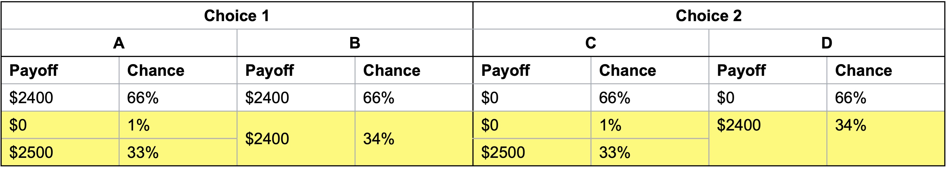
This representation allows us to see that preferring bet B to bet A and bet C to bet D violates the axiom of independence. Under that axiom, two gambles mixed with a third gamble will maintain the same order of preference as when the two are presented independently of the third gamble. In this case, the two gambles are contained in the last two rows. The third gamble is the 66% chance of $2400 or $0. The third gamble is called a “common consequence” as the payoff is the same regardless of whether you choose A or B, or C and D.
I can express this in terms of the formal definition of the independence axiom. The formal definition states that if:
x and y are lotteries with x\succcurlyeq y and
p is the probability that a third option z is present, then:
pz+(1-p)x\succcurlyeq pz+(1-p)y
For each of the choices in our lottery:
x is a 1 in 34 chance of $0 and a 33 in 34 chance of $2500
y is a 100% chance of $2400
z is $2400 in choice 1 and $0 in choice 2.
If p=0, we simply have x\succcurlyeq y. For any non-zero value of p, such as the 66% in both choices, the preference between x and y should not change.
Here’s another intuitive way to think about this bet.
Suppose I am going to generate one number between 1 and 100 randomly.
If a number between 1 and 66 is generated, you win the prize in the first row. If number 67 is generated, you win the amount in the second. If a number from 68 to 100 is generated, you win the sum in the third.
Suppose that you know that the number generated is between 1 and 66. Would you prefer bet A or B in choice 1? As you would win $2400 with either choice, you will be indifferent. You will similarly be indifferent between bet C and D in choice 2, winning $0 no matter what.
Suppose instead that a number between 67 and 100 is generated, but you don’t know which. If you prefer A to B, you should also prefer C to D. In each choice, you effectively face the same bet. Let’s assume for the moment that you prefer A and C.
Finally, suppose you don’t know what number will be generated. We have just determined that if you know the ticket is between 1 and 66, you are indifferent between the options, but if between 67 and 100 is drawn, you prefer A and C. You do not prefer B or D when the ticket range is 1 to 66 or 67 to 100, so you should not prefer B or D when the ticket number is unknown.
However, the responses to the bets generated by Kahneman and Tversky (1979) and many other experimentalists suggest that when the number is unknown, the size of the common consequence for numbers 1 through 66 does matter. This common consequence is changing the preferences of the experimental participants.
11.2 Absurd rates of risk aversion
An important anomaly in expected utility theory concerns the level of risk aversion required to explain observed behaviour.
People reject many small-scale bets. The crux of the anomaly is that if we are expected utility maximisers, rejection implies that we would reject some highly favourable larger-scale bets so favourable almost no one would reject them.
Consider the following one-off bet involving the flip of a coin:
Head: You win $110
Tail: You lose $100
Suppose you reject. You would not be alone in doing this. There is ample evidence that people reject favourable low-stakes bets, even when they have material wealth. Barberis et al. (2006) described an experiment where they offered a 50:50 bet to win $550 or lose $500 to a group of wealthy experimental participants. These participants included clients of a bank’s private wealth management division, with a median wealth above $10 million. Seventy-one percent of the private wealth clients turned down the bet.
Under the axiom of diminishing marginal utility, we could conclude that you rejected it as you are risk averse. However, the minimum utility function curvature required to reconcile an expected utility maximiser declining bets of this nature when you hold any material level of wealth implies that you would reject immensely favourable bets.
Examples in Rabin (2000) and Rabin and Thaler (2001) illustrate this. Suppose a person who acts consistent with expected utility theory always turns down a 50:50 bet to win $110 or lose $100, whatever their wealth. That person will also turn down a 50:50 bet to win $1 billion, lose $1,000. Another expected utility maximiser turns down a 50:50 bet to win $11, lose $10 at all levels of wealth. That person will turn down any 50:50 bet where they could lose $100, no matter the upside.
At face value, that is ridiculous. But that is the crux of the argument. Turning down a low-value bet with a positive expected value implies that the marginal utility of money must decline quickly for small changes in wealth. Rejection of a low-value bet to win $110 or lose $100 would lead to absurd responses to higher-value bets. This leads Rabin (2000) to argue that risk aversion or the diminishing value of money has nothing to do with the rejection of low-value bets.
The intuition behind the rejection of small-scale bets leading to the rejection of immensely favourable bets is as follows.
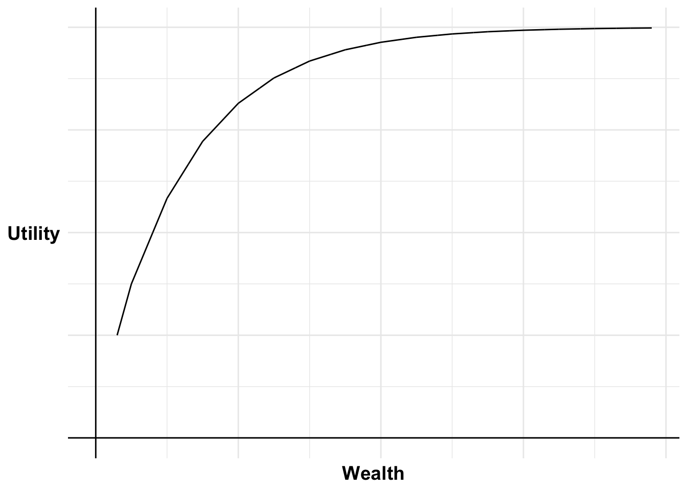
Suppose we have an expected utility maximiser with a weakly concave utility curve. That is, they are risk neutral or risk averse at all levels of wealth. If we drew their utility curve, it would always be increasing at a constant or decreasing rate, depending on where you were on the utility curve.
Code
library(ggplot2)absurdBase <-ggplot(mapping =aes(x, y)) +#Plot the utility curvegeom_vline(xintercept =0, linewidth=0.5)+geom_hline(yintercept =0, linewidth=0.5)+labs(x ="Wealth", y ="Utility")+# Set the themetheme_minimal()+#remove numbers on each axistheme(axis.text.x =element_blank(),axis.text.y =element_blank(),axis.title=element_text(size=14,face="bold"),axis.title.y =element_text(angle=0, vjust=0.5))annotate_plot <-function(plot, W1=250, UW1=3, win=150, loss=100, bets, labels, points=TRUE) {for (i inseq_along(bets)) { bet <- bets[i] label <- labels[i] W <- W1+(win+loss)*(bet-1)if (bet ==1){ UW <- UW1 } else { UW <- UW1for (j in1:(bet-1)) { UW <- UW + (loss/win)^(j-1)+(loss/win)^(j) } }if (label){ plot <- plot +annotate("text", x = W, y =0, label =paste0("W+",W-250), size =3, hjust =0.5, vjust =1.5) }if (label){ plot <- plot +annotate("segment", x = W, y =0, xend = W, yend = UW, linewidth =0.5, colour ="black", linetype="dotted") } plot <- plot +annotate("segment", x = W, y = UW, xend = W-loss, yend = UW-(2/3)^(bet-1), linewidth =0.5, colour ="black") +annotate("segment", x = W, y = UW, xend = W+win, yend = UW+(2/3)^(bet-1), linewidth =0.5, colour ="black")if (points){ plot <- plot +annotate("point", x = W, y = UW, size =2) } }return(plot)}absurd0 <-annotate_plot(absurdBase, bets=c(1:15), labels=rep(FALSE, 15), points=FALSE)absurd0
Figure 11.1: Weakly concave utility curve
This person rejects a 50:50 bet to gain $150, lose $100. (I have chosen this size bet so I can draw this visually to scale and make the point clear. The argument follows the same logic for a win $110, lose $100 bet.) We also assume this person would reject the bet regardless of their level of wealth at the time the bet was offered to them.
I can plot this on a chart. I will develop this chart step by step so that you can understand each element.
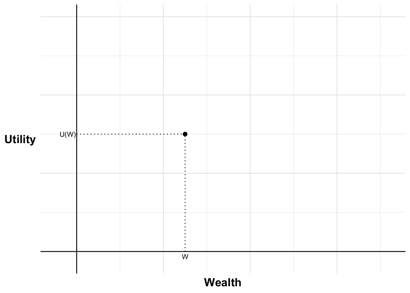
In Figure 11.2, the horizontal axis is wealth and the vertical axis is utility. I have marked the current wealth, W, and utility of that person’s wealth, U(W).
Code
library(ggplot2)W1 <-250win <-150loss <-100UW1=3absurdBase <-ggplot(mapping =aes(x, y)) +#Plot the utility curvegeom_vline(xintercept =0, linewidth=0.5)+geom_hline(yintercept =0, linewidth=0.5)+labs(x ="Wealth", y ="Utility")+# Set the themetheme_minimal()+#remove numbers on each axistheme(axis.text.x =element_blank(),axis.text.y =element_blank(),axis.title=element_text(size=14,face="bold"),axis.title.y =element_text(angle=0, vjust=0.5))absurd1 <- absurdBase+#set limits - need to include room for labelscoord_cartesian(xlim =c(-45, 720), ylim =c(-0.25, 6))+#Add labels W, U(W), dot at W/U(W) and line to curve indicating eachannotate("text", x = W1, y =0, label ="W", size =3, hjust =0.5, vjust =1.5)+annotate("segment", x = W1, y =0, xend = W1, yend = UW1, linewidth =0.5, colour ="black", linetype="dotted")+annotate("segment", x =0, y = UW1, xend = W1, yend = UW1, linewidth =0.5, colour ="black", linetype="dotted")+annotate("text", x =0, y = UW1, label ="U(W)", size =3, hjust =1.05, vjust =0.5)+annotate("point", x = W1, y = UW1, size =2)absurd1
Figure 11.2: Utility of current wealth
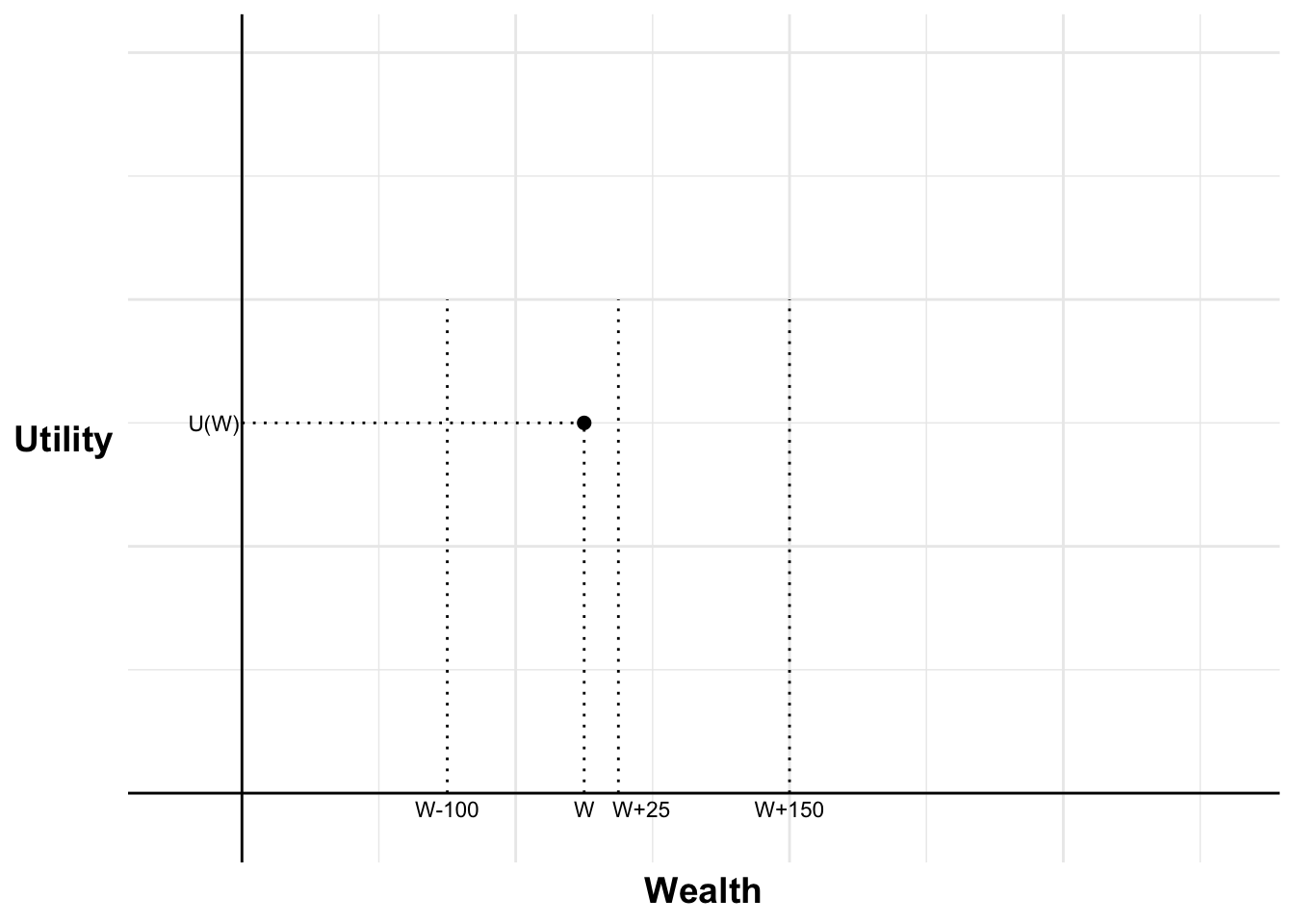
I can then mark in Figure 11.3 the two possible outcomes of the bet, the gain of $150 (W+150) and the loss of $100 (W-100). The utility of each outcome will be a point on these vertical lines.
The expected value of the bet is a gain of $25. That is also marked.
Code
absurd2 <- absurd1+#Add vertical line for the possible win of the first betannotate("segment", x = W1+win, y =0, xend = W1+win, yend =4, linewidth =0.5, colour ="black", linetype="dotted")+annotate("text", x = W1+win, y =0, label ="W+150", size =3, hjust =0.5, vjust =1.5)absurd2+#Add vertical line for the possible loss of the first betannotate("segment", x = W1-loss, y =0, xend = W1-loss, yend =4, linewidth =0.5, colour ="black", linetype="dotted")+annotate("text", x = W1-loss, y =0, label ="W-100", size =3, hjust =0.5, vjust =1.5)+#Add vertical line for the expected value of the first betannotate("segment", x = W1+25, y =0, xend = W1+25, yend =4, linewidth =0.5, colour ="black", linetype="dotted")+annotate("text", x = W1+25, y =0, label ="W+25", size =3, hjust =0.1, vjust =1.5)
Figure 11.3: Outcomes of the bet
As the person rejected the bet, the expected utility of the bet must be less than or equal to the utility of current wealth. The point on the vertical line at W+25 where I mark expected utility must be level with or below the point on the vertical line at W where we mark current utility (U(W)). I have placed a dot on the W+25 line in Figure 11.4 indicating the highest that the expected utility can be.
Code
absurd3 <- absurd2+#Extend line for expected utility of the first bet including dotannotate("segment", x = W1, y = UW1, xend = W1+25, yend = UW1, linewidth =0.5, colour ="black", linetype="dotted")+annotate("point", x = W1+25, y = UW1, size =2)absurd3+#Add vertical line for the possible loss of the first betannotate("segment", x = W1-loss, y =0, xend = W1-loss, yend =4, linewidth =0.5, colour ="black", linetype="dotted")+annotate("text", x = W1-loss, y =0, label ="W-100", size =3, hjust =0.5, vjust =1.5)+#Add vertical line for the expected value of the first betannotate("segment", x = W1+25, y =0, xend = W1+25, yend =4, linewidth =0.5, colour ="black", linetype="dotted")+annotate("text", x = W1+25, y =0, label ="W+25", size =3, hjust =0.1, vjust =1.5)
Figure 11.4: Expected utility of the bet
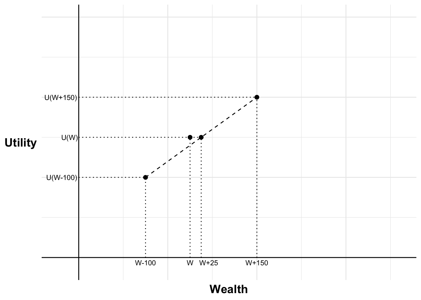
The expected utility of the bet is the probability-weighted utility of each of the two possible outcomes. Therefore, If I draw a line between the utility of each outcome, that line will pass through the expected utility of the bet.
I have added a line in Figure 11.5 between the utility for the two possible outcomes, with the expected utility of the bet on that line (or more specifically, in the middle of the line as each outcome has probability 50%).
Code
absurd4 <- absurd3+#Add line between utility for possible outcomes of the first bet plus dotsannotate("segment", x = W1-loss, y = UW1-1, xend = W1+win, yend = UW1+1, linewidth =0.5, colour ="black", linetype="dashed")+annotate("point", x = W1-loss, y = UW1-1, size =2)+annotate("point", x = W1+win, y = UW1+1, size =2)+#Add vertical line for the possible loss of the first betannotate("segment", x = W1-loss, y =0, xend = W1-loss, yend =2, linewidth =0.5, colour ="black", linetype="dotted")+annotate("text", x = W1-loss, y =0, label ="W-100", size =3, hjust =0.5, vjust =1.5)+#Add vertical line for the expected value of the first betannotate("segment", x = W1+25, y =0, xend = W1+25, yend =3, linewidth =0.5, colour ="black", linetype="dotted")+annotate("text", x = W1+25, y =0, label ="W+25", size =3, hjust =0.1, vjust =1.5)+#Add horizontal line for U(W+150) and U(W-100) and expected valueannotate("segment", x =0, y = UW1+1, xend = W1+150, yend = UW1+1, linewidth =0.5, colour ="black", linetype="dotted")+annotate("text", x =0, y = UW1+1, label ="U(W+150)", size =3, hjust =1.05, vjust =0.5)+annotate("segment", x =0, y = UW1-1, xend = W1-loss, yend = UW1-1, linewidth =0.5, colour ="black", linetype="dotted")+annotate("text", x =0, y = UW1-1, label ="U(W-100)", size =3, hjust =1.05, vjust =0.5)absurd4
Figure 11.5: Utility of the outcomes of the bet
We now have three points on the utility curve: current wealth and their utility if the person lost or won the bet.
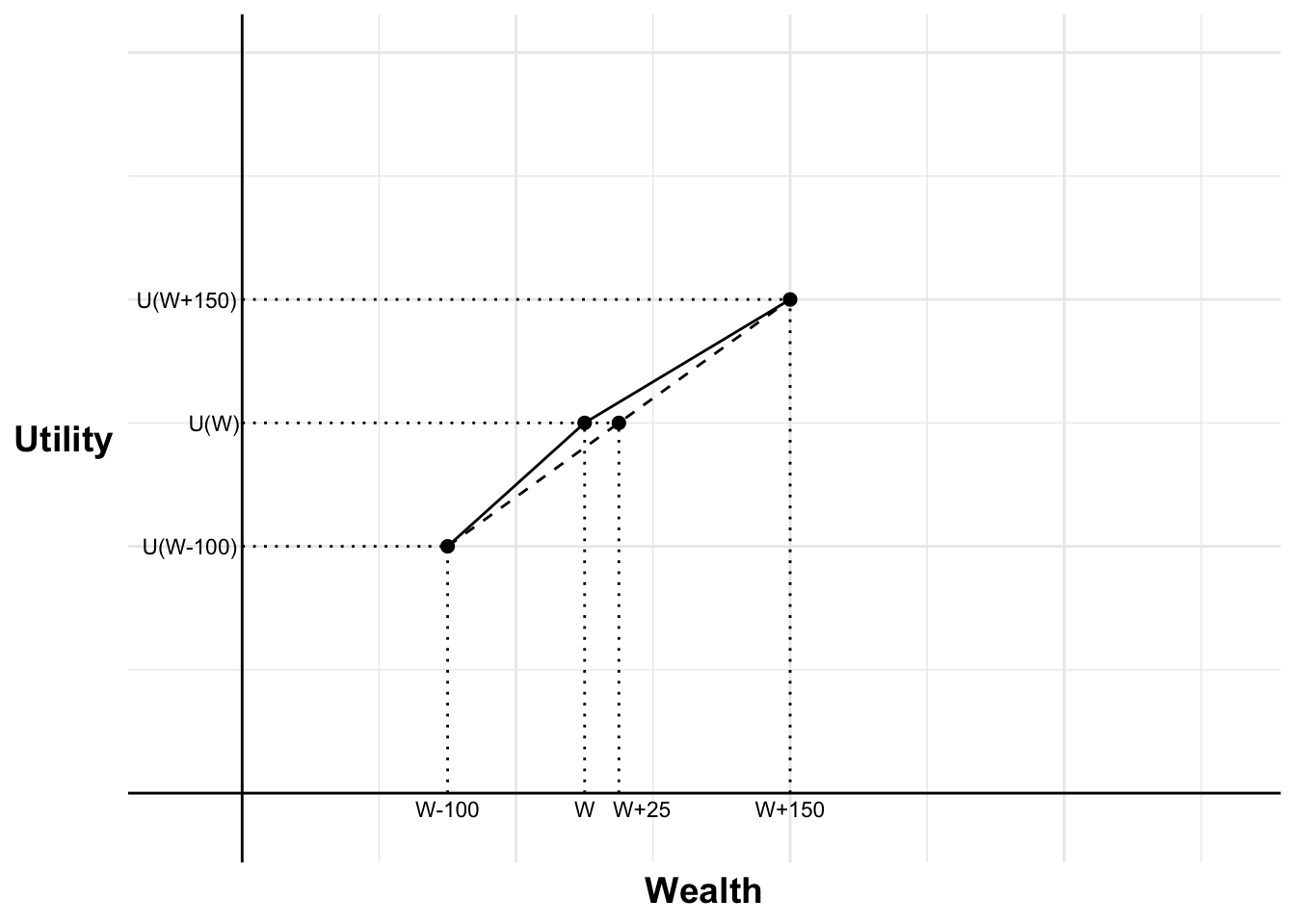
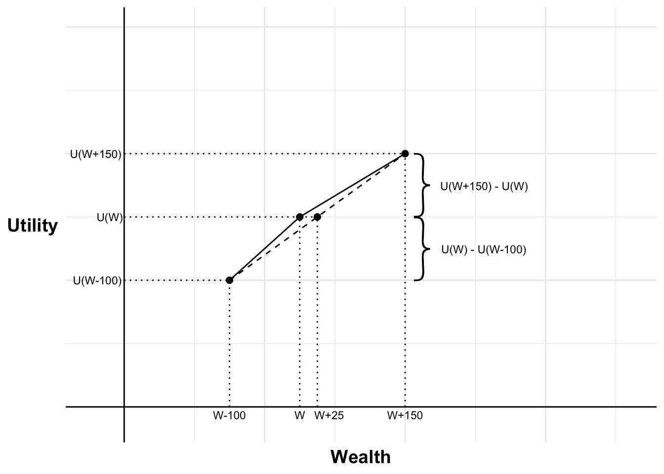
As the person is risk averse at all levels of wealth, we know that all parts of the utility curve are at a minimum weakly concave. We can therefore draw in Figure 11.6 part of the utility curve as the least risk averse they could be while still rejecting the bet. This is drawn in the solid black line.
Code
absurd5 <- absurd4+#Add line linking the utility of the two first bet outcomes and utility of current wealthannotate("segment", x = W1, y = UW1, xend = W1-loss, yend = UW1-1, linewidth =0.5, colour ="black")+annotate("segment", x = W1, y = UW1, xend = W1+win, yend = UW1+1, linewidth =0.5, colour ="black")absurd5
Figure 11.6: Utility curve
From the rejection of the bet, we know that:
U(W+150)-U(W)\leq U(W)-U(W-100)
Code
absurd5a <- absurd5+#add curly bracket indicating increase in utility with winannotate("text", x =425, y =3.44, label ='{', angle =180, size =20, family ='Source Sans Pro ExtraLight')+annotate("text", x =500, y =3.62, label ="U(W+150) - U(W)", size =3, hjust =0.4, vjust =1.5)+#add curly bracket indicating decrease in utility with lossannotate("text", x =425, y =2.44, label ='{', angle =180, size =20, family ='Source Sans Pro ExtraLight')+annotate("text", x =500, y =2.62, label ="U(W) - U(W-100)", size =3, hjust =0.4, vjust =1.5)absurd5a
Figure 11.7: Utility curve
This means that you value each dollar between W and W+150, on average, by at most 100/150ths (or 2/3rds) as much as you value each dollar, on average, between W and W-100. We can see this in the slope of the two black lines forming the part of the utility curve we have drawn. The second part has two thirds the slope of the first.
Further, by weak concavity, we can say that you value your W+150th dollar at most two thirds as much as you value your W-100th dollar. The relative value of each dollar has declined by at least one third over the span of $250.
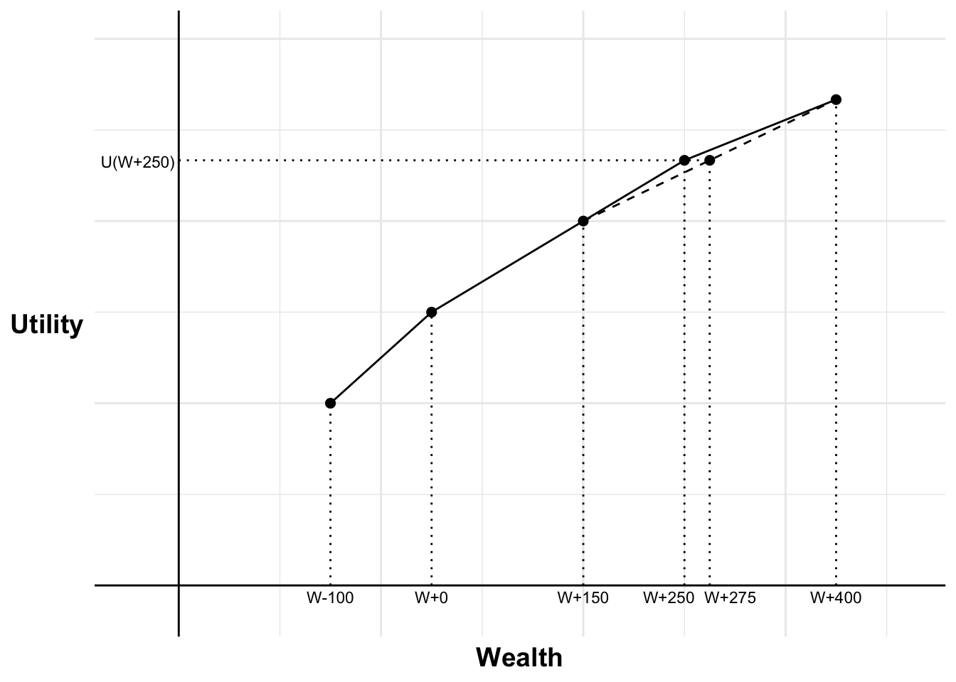
Let us now consider what would happen if this person had $250 more wealth: that is, they have W+250. They are then offered the same bet.
We have assumed that they will reject the bet at all levels of wealth, so they will also reject at this wealth. We can, therefore, infer another piece of the utility curve (or, more specifically, a curve for the least risk averse they could be). I have marked in Figure 11.8 the utility of their wealth, the highest the expected utility of the bet can be if they reject the bet, and the utility of the two possible outcomes of the bet. The next section of solid black line represents another part of the utility curve that is at the minimum risk aversion they could be while still rejecting the bet.
Code
W2 <- W1 +250UW2 <- UW1 +1+2/3absurd6 <-annotate_plot(absurdBase, bets=c(1, 2), labels=c(TRUE, FALSE))absurd6+#Add horizontal line for U(W2) and expected valueannotate("segment", x =0, y = UW2, xend = W2+25, yend = UW2, linewidth =0.5, colour ="black", linetype="dotted")+annotate("text", x =0, y = UW2, label ="U(W+250)", size =3, hjust =1.05, vjust =0.6)+#Add vertical line and dot for the possible win of the first betannotate("segment", x = W1+win, y =0, xend = W1+win, yend = UW1+1, linewidth =0.5, colour ="black", linetype="dotted")+annotate("text", x = W1+win, y =0, label ="W+150", size =3, hjust =0.5, vjust =1.5)+annotate("point", x = W1+win, y = UW1+1, size =2)+#Add vertical line and dot for the possible loss of the first betannotate("segment", x = W1-loss, y =0, xend = W1-loss, yend = UW1-1, linewidth =0.5, colour ="black", linetype="dotted")+annotate("text", x = W1-loss, y =0, label ="W-100", size =3, hjust =0.5, vjust =1.5)+annotate("point", x = W1-loss, y = UW1-1, size =2)+#Add labels and line W+250 - doing here as want to remove laterannotate("text", x = W2, y =0, label ="W+250", size =3, hjust =0.8, vjust =1.5)+annotate("segment", x = W2, y =0, xend = W2, yend = UW2, linewidth =0.5, colour ="black", linetype="dotted")+#Add vertical line for the possible win of the second bet, including a dotannotate("segment", x = W2+150, y =0, xend = W2+150, yend = UW2+2/3, linewidth =0.5, colour ="black", linetype="dotted")+annotate("point", x = W2+150, y =5.333, size =2)+annotate("text", x = W2+150, y =0, label ="W+400", size =3, hjust =0.5, vjust =1.5)+#Add line linking for the expected utility of the two second bet outcomesannotate("segment", x = W2-100, y = UW2-2/3, xend = W2+150, yend = UW2+2/3, linewidth =0.5, colour ="black", linetype="dashed")+#Add vertical line and dot for the expected value of the second betannotate("segment", x = W2+25, y =0, xend = W2+25, yend = UW2, linewidth =0.5, colour ="black", linetype="dotted")+annotate("text", x = W2+25, y =0, label ="W+275", size =3, hjust =0.1, vjust =1.5)+annotate("point", x = W2+25, y = UW2, size =2)+#set limits - need to include room for labelscoord_cartesian(xlim =c(-45, 720), ylim =c(-0.25, 6))
Figure 11.8: Utility curve extended
Iterating the previous calculations, I can say that they will weight their W+400th dollar only two thirds as much as their W+150th dollar. This means they value their W+400th dollar only (2/3)2 or 4/9 as much as their W-100th dollar. Or put another way, over the span of $500, the relative value of each dollar has declined by five ninths.
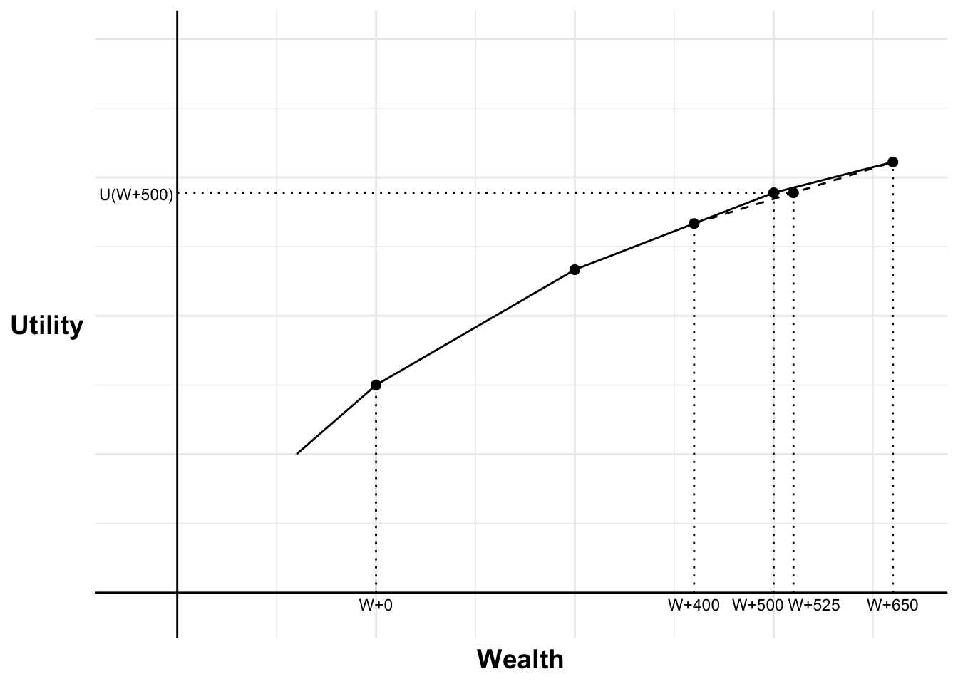
As we infer additional pieces, we can see in Figure 11.9 that this person rapidly declines in the rate at which they place utility on further wealth. The increase in slope for each additional sum becomes less and less.
Code
W3 <- W2 +250UW3 <- UW2 +2/3+4/9absurd7 <-annotate_plot(absurd6, bets=c(3), labels=c(FALSE))+annotate("segment", x = W3, y =0, xend = W3, yend = UW3, linewidth =0.5, colour ="black", linetype="dotted")absurd7+#Add line for U(W2) and expected valueannotate("segment", x =0, y = UW3, xend = W3+25, yend = UW3, linewidth =0.5, colour ="black", linetype="dotted")+annotate("text", x =0, y = UW3, label ="U(W+500)", size =3, hjust =1.05, vjust =0.6)+#Add labels W+500 - doing here so can centre laterannotate("text", x = W3, y =0, label ="W+500", size =3, hjust =0.8, vjust =1.5)+#Add vertical line for the possible win of the second bet, including a dotannotate("segment", x = W2+150, y =0, xend = W2+150, yend = UW2+2/3, linewidth =0.5, colour ="black", linetype="dotted")+annotate("point", x = W2+150, y =5.333, size =2)+annotate("text", x = W2+150, y =0, label ="W+400", size =3, hjust =0.5, vjust =1.5)+#Add vertical line and dot for the possible win of the third betannotate("segment", x = W3+win, y =0, xend = W3+win, yend = UW3+4/9, linewidth =0.5, colour ="black", linetype="dotted")+annotate("text", x = W3+win, y =0, label ="W+650", size =3, hjust =0.5, vjust =1.5)+annotate("point", x = W3+win, y = UW3+4/9, size =2)+#Add line linking for the expected utility of the two third bet outcomesannotate("segment", x = W3-100, y = UW3-4/9, xend = W3+150, yend = UW3+4/9, linewidth =0.5, colour ="black", linetype="dashed")+#Add vertical line and dot for the expected value of the third betannotate("segment", x = W3+25, y =0, xend = W3+25, yend = UW3, linewidth =0.5, colour ="black", linetype="dotted")+annotate("text", x = W3+25, y =0, label ="W+525", size =3, hjust =0.1, vjust =1.5)+annotate("point", x = W3+25, y = UW3, size =2)+#set limits - need to include room for labelscoord_cartesian(xlim =c(-55, 920), ylim =c(-0.25, 8))
Figure 11.9: Utility curve further extended
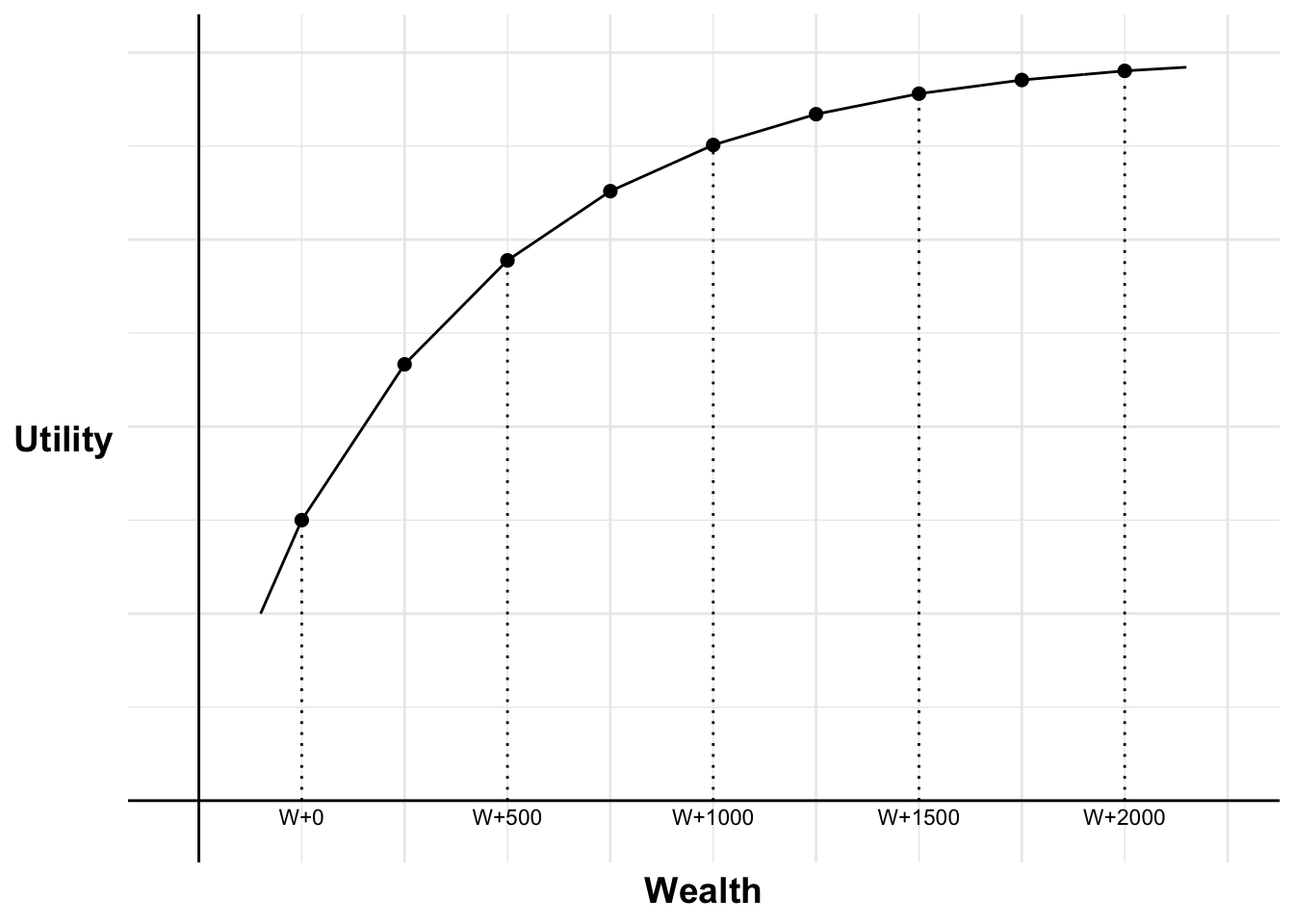
Over time, the slope approaches a horizontal asymptote: effectively, a cap on the level of utility they can achieve, however wealthy they may become. This is shown in Figure 11.10.
Code
absurd8 <-annotate_plot(absurd7, bets=c(4, 5, 6, 7, 8, 9), labels=c(FALSE, TRUE, FALSE, TRUE, FALSE, TRUE))+#Add labels W+500annotate("text", x = W3, y =0, label ="W+500", size =3, hjust =0.5, vjust =1.5)absurd8+#set limits - need to include room for labelscoord_cartesian(xlim =c(-45, 2500), ylim =c(-0.25, 8))
Figure 11.10: Utility curve asymptote
Keep iterating in this way and you end up with some ridiculous results. You value the 2500th dollar above your current wealth only 2% as much as your last current dollar of your wealth - (2/3)10 - reducing by a constant factor of 2/3 every $250. This is an absurd rate of discounting.
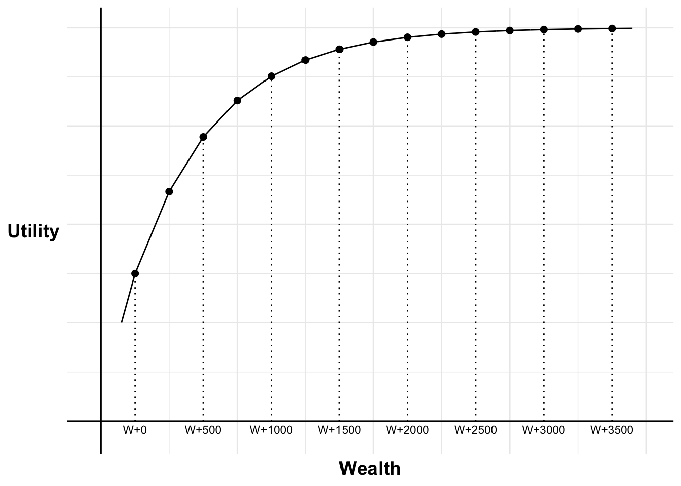
Taking this iteration to the extreme, it doesn’t take long for additional money to have effectively zero value. In Figure 11.11, we see the utility curve approaching a limit. Any gain of money from W+3000 upwards is valued at almost nothing, meaning a gain beyond that level, no matter how large, could compensate for the possibility of losing $1,000.
Code
absurd9 <-annotate_plot(absurd8, bets=c(10, 11, 12, 13, 14,15), labels=c(FALSE, TRUE, FALSE, TRUE, FALSE, TRUE))absurd9 +#set limits - need to include room for labelscoord_cartesian(xlim =c(-45, 4000), ylim =c(-0.25, 8))
Figure 11.11: Utility curve limit
11.3 Framing
Under expected utility theory, a person’s choices should not be affected by how the options are described or by how their preferences are elicited.
Kahneman and Tversky (1984) reported the following experiment.
A group of experimental participants were shown the following:
Imagine that the U.S. is preparing for the outbreak of an unusual Asian disease, which is expected to kill 600 people. Two alternative programs to combat the disease have been proposed. Assume that the exact scientific estimates of the consequences of the programs are as follows:
If Program A is adopted, 200 people will be saved.
If Program B is adopted, there is a one-third probability that 600 people will be saved and a two-thirds probability that no people will be saved.
Which of the two programs would you favour?
72% of participants chose option A.
Another group of experimental participants were shown the following:
Imagine that the U.S. is preparing for the outbreak of an unusual Asian disease, which is expected to kill 600 people. Two alternative programs to combat the disease have been proposed. Assume that the exact scientific estimates of the consequences of the programs are as follows:
If Program C is adopted, 400 people will die.
If Program D is adopted, there is a one-third probability that nobody will die and a two-thirds probability that 600 people will die.
Which of the two programs would you favour?
22% of participants chose option C.
72% of participants chose A and 22% of participants chose option C. Yet these two options are equivalent. The only difference is the framing of the options, which under expected utility theory should not matter.
11.4 Reference points
An auxiliary axiom of expected utility theory is that people use a reference point of zero wealth. They consider the utility of the absolute outcomes.
However, consider the following two scenarios:
You have not checked your share portfolio in a while. You expect that the portfolio is worth around $40,000. Today when you check, it is worth $30,000. Do you feel rich or poor?
You have not checked your share portfolio in a while. You expect that the portfolio is worth around $20,000. Today when you check, it is worth $30,000. Do you feel rich or poor?
Under expected utility theory, those two scenarios should feel the same as you have U(\$30,000) in both cases.
However, in the first case, you feel poor and in the second case you feel rich. This is because you are comparing the outcome to your reference point of $40,000 in the first case and $20,000 in the second case. You are not assessing the absolute outcome but appear to be using a reference point.
That is, U(W) \neq U(W') when W = W' but reference points differ.
Allais, M. (1953). Le comportement de l’homme rationnel devant le risque: Critique des postulats et axiomes de l’ecole americaine. Econometrica, 21(4), 503–546. https://doi.org/10.2307/1907921
Barberis, N., Huang, M., and Thaler, R. H. (2006). Individual Preferences, Monetary Gambles, and Stock Market Participation: A Case for Narrow Framing. American Economic Review, 96(4), 1069–1090. https://doi.org/10.1257/aer.96.4.1069
Kahneman, D., and Tversky, A. (1979). Prospect theory: An analysis of decision under risk. Econometrica, 47(2), 263–291. https://doi.org/10.2307/1914185
Rabin, M. (2000). Risk Aversion and Expected-Utility Theory: A Calibration Theorem. Econometrica, 68(5), 1281–1292. http://www.jstor.org/stable/2999450
Rabin, M., and Thaler, R. H. (2001). Anomalies: Risk Aversion. Journal of Economic Perspectives, 15(1), 219–232. https://doi.org/10.1257/jep.15.1.219